# index.html.md
# NVIDIA NIM Microservices
## Natural Language Processing
NeMo Retriever
Get access to state-of-the-art models for building text Q&A retrieval pipelines with high accuracy.
Text Embedding
Text Reranking
# index.html.md
# Local
Choose your preferred installation method for running RAPIDS
Conda
Install RAPIDS using conda
Docker
Install RAPIDS using Docker
pip
Install RAPIDS using pip
WSL2
Install RAPIDS on Windows using Windows Subsystem for Linux version 2 (WSL2)
# index.html.md
# HPC
RAPIDS works extremely well in traditional HPC (High Performance Computing) environments where GPUs are often co-located with accelerated networking hardware such as InfiniBand. Deploying on HPC often means using queue management systems such as SLURM, LSF, PBS, etc.
## SLURM
#### WARNING
This is a legacy page and may contain outdated information. We are working hard to update our documentation with the latest and greatest information, thank you for bearing with us.
If you are unfamiliar with SLURM or need a refresher, we recommend the [quickstart guide](https://slurm.schedmd.com/quickstart.html).
Depending on how your nodes are configured, additional settings may be required such as defining the number of GPUs `(--gpus)` desired or the number of gpus per node `(--gpus-per-node)`.
In the following example, we assume each allocation runs on a DGX1 with access to all eight GPUs.
### Start Scheduler
First, start the scheduler with the following SLURM script. This and the following scripts can deployed with `salloc` for interactive usage or `sbatch` for batched run.
```bash
#!/usr/bin/env bash
#SBATCH -J dask-scheduler
#SBATCH -n 1
#SBATCH -t 00:10:00
module load cuda/11.0.3
CONDA_ROOT=/nfs-mount/user/miniconda3
source $CONDA_ROOT/etc/profile.d/conda.sh
conda activate rapids
LOCAL_DIRECTORY=/nfs-mount/dask-local-directory
mkdir $LOCAL_DIRECTORY
CUDA_VISIBLE_DEVICES=0 dask-scheduler \
--protocol tcp \
--scheduler-file "$LOCAL_DIRECTORY/dask-scheduler.json" &
dask-cuda-worker \
--rmm-pool-size 14GB \
--scheduler-file "$LOCAL_DIRECTORY/dask-scheduler.json"
```
Notice that we configure the scheduler to write a `scheduler-file` to a NFS accessible location. This file contains metadata about the scheduler and will
include the IP address and port for the scheduler. The file will serve as input to the workers informing them what address and port to connect.
The scheduler doesn’t need the whole node to itself so we can also start a worker on this node to fill out the unused resources.
### Start Dask CUDA Workers
Next start the other [dask-cuda workers](https://docs.rapids.ai/api/dask-cuda/nightly/). Dask-CUDA extends the traditional Dask `Worker` class with specific options and enhancements for GPU environments. Unlike the scheduler and client, the workers script should be scalable and allow the users to tune how many workers are created.
For example, we can scale the number of nodes to 3: `sbatch/salloc -N3 dask-cuda-worker.script` . In this case, because we have 8 GPUs per node and we have 3 nodes,
our job will have 24 workers.
```bash
#!/usr/bin/env bash
#SBATCH -J dask-cuda-workers
#SBATCH -t 00:10:00
module load cuda/11.0.3
CONDA_ROOT=/nfs-mount/miniconda3
source $CONDA_ROOT/etc/profile.d/conda.sh
conda activate rapids
LOCAL_DIRECTORY=/nfs-mount/dask-local-directory
mkdir $LOCAL_DIRECTORY
dask-cuda-worker \
--rmm-pool-size 14GB \
--scheduler-file "$LOCAL_DIRECTORY/dask-scheduler.json"
```
### cuDF Example Workflow
Lastly, we can now run a job on the established Dask Cluster.
```bash
#!/usr/bin/env bash
#SBATCH -J dask-client
#SBATCH -n 1
#SBATCH -t 00:10:00
module load cuda/11.0.3
CONDA_ROOT=/nfs-mount/miniconda3
source $CONDA_ROOT/etc/profile.d/conda.sh
conda activate rapids
LOCAL_DIRECTORY=/nfs-mount/dask-local-directory
cat <>/tmp/dask-cudf-example.py
import cudf
import dask.dataframe as dd
from dask.distributed import Client
client = Client(scheduler_file="$LOCAL_DIRECTORY/dask-scheduler.json")
cdf = cudf.datasets.timeseries()
ddf = dd.from_pandas(cdf, npartitions=10)
res = ddf.groupby(['id', 'name']).agg(['mean', 'sum', 'count']).compute()
print(res)
EOF
python /tmp/dask-cudf-example.py
```
### Confirm Output
Putting the above together will result in the following output:
```bash
x y
mean sum count mean sum count
id name
1077 Laura 0.028305 1.868120 66 -0.098905 -6.527731 66
1026 Frank 0.001536 1.414839 921 -0.017223 -15.862306 921
1082 Patricia 0.072045 3.602228 50 0.081853 4.092667 50
1007 Wendy 0.009837 11.676199 1187 0.022978 27.275216 1187
976 Wendy -0.003663 -3.267674 892 0.008262 7.369577 892
... ... ... ... ... ... ...
912 Michael 0.012409 0.459119 37 0.002528 0.093520 37
1103 Ingrid -0.132714 -1.327142 10 0.108364 1.083638 10
998 Tim 0.000587 0.747745 1273 0.001777 2.262094 1273
941 Yvonne 0.050258 11.358393 226 0.080584 18.212019 226
900 Michael -0.134216 -1.073729 8 0.008701 0.069610 8
[6449 rows x 6 columns]
```
# index.html.md
# Continuous Integration
GitHub Actions
Run tests in GitHub Actions that depend on RAPIDS and NVIDIA GPUs.
single-node
# index.html.md
# Custom RAPIDS Docker Guide
This guide provides instructions for building custom RAPIDS Docker containers. This approach allows you to select only the RAPIDS libraries you need, which is ideal for creating minimal, customizable images that can be tuned to your requirements.
#### NOTE
For quick setup with pre-built containers that include the full RAPIDS suite, please see the [Official RAPIDS Docker Installation Guide](https://docs.rapids.ai/install#docker).
## Overview
Building a custom RAPIDS container offers several advantages:
- **Minimal Image Sizes**: By including only the libraries you need, you can reduce the final image size.
- **Flexible Configuration**: You have full control over library versions and dependencies.
## Getting Started
To begin, you will need to create a few local files for your custom build: a `Dockerfile` and a configuration file (`env.yaml` for conda or `requirements.txt` for pip). The templates for these files is provided in the Docker Templates section below for you to copy.
1. **Create a Project Directory**: It’s best practice to create a dedicated folder for your custom build.
```bash
mkdir rapids-custom-build && cd rapids-custom-build
```
2. **Prepare Your Project Files**: Based on your chosen approach (conda or pip), create the necessary files in your project directory from the corresponding tab in the Docker Templates section below.
3. **Customize Your Build**:
- When using **conda**, edit your local `env.yaml` file to add the desired RAPIDS libraries.
- When using **pip**, edit your local `requirements.txt` file with your desired RAPIDS libraries.
4. **Build the Image**: Use the commands provided in the Build and Run section to create and start your custom container.
---
## Package Manager Differences
The choice of base image depends on how your package manager handles CuPy (a dependency for most RAPIDS libraries) and CUDA library dependencies:
### Conda → Uses `cuda-base`
```dockerfile
FROM nvidia/cuda:12.9.1-base-ubuntu24.04
```
This approach works because conda can install both Python and non-Python dependencies, including system-level CUDA libraries like `libcudart` and `libnvrtc`. When installing RAPIDS libraries via conda, the package manager automatically pulls the required CUDA runtime libraries alongside CuPy and other dependencies, providing complete dependency management in a single installation step.
### Pip → Uses `cuda-runtime`
```dockerfile
FROM nvidia/cuda:12.9.1-runtime-ubuntu24.04
```
This approach is necessary because CuPy wheels distributed via PyPI do not currently bundle CUDA runtime libraries (`libcudart`, `libnvrtc`) within the wheel packages themselves. Since pip cannot install system-level CUDA libraries, CuPy expects these libraries to already be present in the system environment. The `cuda-runtime` image provides the necessary CUDA runtime libraries that CuPy requires, eliminating the need for manual library installation.
## Docker Templates
The complete source code for the Dockerfiles and their configurations are included here. Choose your preferred package manager.
### conda
This method uses conda and is ideal for workflows that are based on `conda`.
**`rapids-conda.Dockerfile`**
```dockerfile
# syntax=docker/dockerfile:1
# Copyright (c) 2024-2025, NVIDIA CORPORATION.
ARG CUDA_VER=12.9.1
ARG LINUX_DISTRO=ubuntu
ARG LINUX_DISTRO_VER=24.04
FROM nvidia/cuda:${CUDA_VER}-base-${LINUX_DISTRO}${LINUX_DISTRO_VER}
SHELL ["/bin/bash", "-euo", "pipefail", "-c"]
# Install system dependencies
RUN apt-get update && \
apt-get install -y --no-install-recommends \
wget \
curl \
git \
ca-certificates \
&& rm -rf /var/lib/apt/lists/*
# Install Miniforge
RUN wget -qO /tmp/miniforge.sh "https://github.com/conda-forge/miniforge/releases/latest/download/Miniforge3-Linux-x86_64.sh" && \
bash /tmp/miniforge.sh -b -p /opt/conda && \
rm /tmp/miniforge.sh && \
/opt/conda/bin/conda clean --all --yes
# Add conda to PATH and activate base environment
ENV PATH="/opt/conda/bin:${PATH}"
ENV CONDA_DEFAULT_ENV=base
ENV CONDA_PREFIX=/opt/conda
# Create conda group and rapids user
RUN groupadd -g 1001 conda && \
useradd -rm -d /home/rapids -s /bin/bash -g conda -u 1001 rapids && \
chown -R rapids:conda /opt/conda
USER rapids
WORKDIR /home/rapids
# Copy the environment file template
COPY --chmod=644 env.yaml /home/rapids/env.yaml
# Update the base environment with user's packages from env.yaml
# Note: The -n base flag ensures packages are installed to the base environment
# overriding any 'name:' specified in the env.yaml file
RUN /opt/conda/bin/conda env update -n base -f env.yaml && \
/opt/conda/bin/conda clean --all --yes
CMD ["bash"]
```
**`env.yaml`** (Conda environment configuration)
```yaml
name: base
channels:
- "rapidsai-nightly"
- conda-forge
- nvidia
dependencies:
- python=3.12
- cudf=25.12
```
### pip
This approach uses Python virtual environments and is ideal for workflows that are already based on `pip`.
**`rapids-pip.Dockerfile`**
```dockerfile
# syntax=docker/dockerfile:1
# Copyright (c) 2024-2025, NVIDIA CORPORATION.
ARG CUDA_VER=12.9.1
ARG PYTHON_VER=3.12
ARG LINUX_DISTRO=ubuntu
ARG LINUX_DISTRO_VER=24.04
# Use CUDA runtime image for pip
FROM nvidia/cuda:${CUDA_VER}-runtime-${LINUX_DISTRO}${LINUX_DISTRO_VER}
ARG PYTHON_VER
SHELL ["/bin/bash", "-euo", "pipefail", "-c"]
# Install system dependencies
RUN apt-get update && \
apt-get install -y --no-install-recommends \
python${PYTHON_VER} \
python${PYTHON_VER}-venv \
python3-pip \
wget \
curl \
git \
ca-certificates \
&& rm -rf /var/lib/apt/lists/*
# Create symbolic links for python and pip
RUN ln -sf /usr/bin/python${PYTHON_VER} /usr/bin/python && \
ln -sf /usr/bin/python${PYTHON_VER} /usr/bin/python3
# Create rapids user
RUN groupadd -g 1001 rapids && \
useradd -rm -d /home/rapids -s /bin/bash -g rapids -u 1001 rapids
USER rapids
WORKDIR /home/rapids
# Create and activate virtual environment
RUN python -m venv /home/rapids/venv
ENV PATH="/home/rapids/venv/bin:$PATH"
ENV VIRTUAL_ENV="/home/rapids/venv"
# Upgrade pip
RUN pip install --no-cache-dir --upgrade pip setuptools wheel
# Copy the requirements file
COPY --chmod=644 requirements.txt /home/rapids/requirements.txt
# Install all packages
RUN pip install --no-cache-dir -r requirements.txt
CMD ["bash"]
```
**`requirements.txt`** (Pip package requirements)
```text
# RAPIDS libraries (pip versions)
cudf-cu12==25.12.*,>=0.0.0a0
```
---
## Build and Run
### Conda
After copying the source files into your local directory:
```bash
# Build the image
docker build -f rapids-conda.Dockerfile -t rapids-conda-base .
# Start a container with an interactive shell
docker run --gpus all -it rapids-conda-base
```
### Pip
After copying the source files into your local directory:
```bash
# Build the image
docker build -f rapids-pip.Dockerfile -t rapids-pip-base .
# Start a container with an interactive shell
docker run --gpus all -it rapids-pip-base
```
#### IMPORTANT
When using `pip`, you must specify the CUDA version in the package name (e.g., `cudf-cu12`, `cuml-cu12`). This ensures you install the version of the library that is compatible with the CUDA toolkit.
#### NOTE
**GPU Access with `--gpus all`**: The `--gpus` flag uses the NVIDIA Container Toolkit to dynamically mount GPU device files (`/dev/nvidia*`), NVIDIA driver libraries (`libcuda.so`, `libnvidia-ml.so`), and utilities like `nvidia-smi` from the host system into your container at runtime. This is why `nvidia-smi` becomes available even though it’s not installed in your Docker image. Your container only needs to provide the CUDA runtime libraries (like `libcudart`) that RAPIDS requires—the host system’s NVIDIA driver handles the rest.
### Image Size Comparison
One of the key benefits of building custom RAPIDS containers is the significant reduction in image size compared to the pre-built RAPIDS images. Here are actual measurements from containers containing only cuDF:
| Image Type | Contents | Size |
|----------------------|-------------------|-------------|
| **Custom conda** | cuDF only | **6.83 GB** |
| **Custom pip** | cuDF only | **6.53 GB** |
| **Pre-built RAPIDS** | Full RAPIDS suite | **12.9 GB** |
Custom builds are smaller in size when you only need specific RAPIDS libraries like cuDF. These size reductions result in faster container pulls and deployments, reduced storage costs in container registries, lower bandwidth usage in distributed environments, and quicker startup times for containerized applications.
## Extending the Container
One of the benefits of building custom RAPIDS containers is the ability to easily add your own packages to the environment. You can add any combination of RAPIDS and non-RAPIDS libraries to create a fully featured container for your workloads.
### Using conda
To add packages to the Conda environment, add them to the `dependencies` list in your `env.yaml` file.
**Example: Adding `scikit-learn` and `xgboost` to a conda image containing `cudf`**
```yaml
name: base
channels:
- rapidsai-nightly
- conda-forge
- nvidia
dependencies:
- cudf=25.12
- scikit-learn
- xgboost
```
### Using pip
To add packages to the Pip environment, add them to your `requirements.txt` file.
**Example: Adding `scikit-learn` and `lightgbm` to a pip image containing `cudf`**
```text
cudf-cu12==25.12.*,>=0.0.0a0
scikit-learn
lightgbm
```
After modifying your configuration file, rebuild the Docker image. The new packages will be automatically included in your custom RAPIDS environment.
## Build Configuration
You can customize the build by modifying the version variables at the top of each Dockerfile. These variables control the CUDA version, Python version, and Linux distribution used in your container.
### Available Configuration Variables
The following variables can be modified at the top of each Dockerfile to customize your build:
| Variable | Default Value | Description | Example Values |
|-------------------------|-----------------|--------------------------------------------------------|----------------------|
| `CUDA_VER` | `12.9.1` | Sets the CUDA version for the base image and packages. | `12.0` |
| `PYTHON_VER` (pip only) | `3.12` | Defines the Python version to install and use. | `3.11`, `3.10` |
| `LINUX_DISTRO` | `ubuntu` | The Linux distribution being used | `rockylinux9`, `cm2` |
| `LINUX_DISTRO_VER` | `24.04` | The version of the Linux distribution. | `20.04` |
#### NOTE
For conda installations, you can choose the required python version in the `env.yaml` file
## Verifying Your Installation
After starting your container, you can quickly test that RAPIDS is installed and running correctly. The container launches directly into a `bash` shell where you can install the [RAPIDS CLI](https://github.com/rapidsai/rapids-cli) command line utility to verify your installation.
1. **Run the Container Interactively**
This command starts your container and drops you directly into a bash shell.
```bash
# For Conda builds
docker run --gpus all -it rapids-conda-base
# For Pip builds
docker run --gpus all -it rapids-pip-base
```
2. **Install RAPIDS CLI**
Inside the containers, install the RAPIDS CLI:
```bash
pip install rapids-cli
```
3. **Test the installation using the Doctor subcommand**
Once RAPIDS CLI is installed, you can use the `rapids doctor` subcommand to perform health checks.
```bash
rapids doctor
```
4. **Expected Output**
If your installation is successful, you will see output similar to this:
```bash
🧑⚕️ Performing REQUIRED health check for RAPIDS
Running checks
All checks passed!
```
# index.html.md
# Continuous Integration
GitHub Actions
Run tests in GitHub Actions that depend on RAPIDS and NVIDIA GPUs.
single-node
# index.html.md
To access Jupyter, navigate to `:8888` in the browser.
In a Python notebook, check that you can import and use RAPIDS libraries like `cudf`.
```ipython
In [1]: import cudf
In [2]: df = cudf.datasets.timeseries()
In [3]: df.head()
Out[3]:
id name x y
timestamp
2000-01-01 00:00:00 1020 Kevin 0.091536 0.664482
2000-01-01 00:00:01 974 Frank 0.683788 -0.467281
2000-01-01 00:00:02 1000 Charlie 0.419740 -0.796866
2000-01-01 00:00:03 1019 Edith 0.488411 0.731661
2000-01-01 00:00:04 998 Quinn 0.651381 -0.525398
```
Open `cudf/10min.ipynb` and execute the cells to explore more of how `cudf` works.
When running a Dask cluster you can also visit `:8787` to monitor the Dask cluster status.
# index.html.md
Let’s create a sample Pod that uses some GPU compute to make sure that everything is working as expected.
```bash
cat << EOF | kubectl create -f -
apiVersion: v1
kind: Pod
metadata:
name: cuda-vectoradd
spec:
restartPolicy: OnFailure
containers:
- name: cuda-vectoradd
image: "nvidia/samples:vectoradd-cuda11.6.0-ubuntu18.04"
resources:
limits:
nvidia.com/gpu: 1
EOF
```
```console
$ kubectl logs pod/cuda-vectoradd
[Vector addition of 50000 elements]
Copy input data from the host memory to the CUDA device
CUDA kernel launch with 196 blocks of 256 threads
Copy output data from the CUDA device to the host memory
Test PASSED
Done
```
If you see `Test PASSED` in the output, you can be confident that your Kubernetes cluster has GPU compute set up correctly.
Next, clean up that Pod.
```console
$ kubectl delete pod cuda-vectoradd
pod "cuda-vectoradd" deleted
```
# index.html.md
There are a selection of methods you can use to install RAPIDS which you can see via the [RAPIDS release selector](https://docs.rapids.ai/install#selector).
For this example we are going to run the RAPIDS Docker container so we need to know the name of the most recent container.
On the release selector choose **Docker** in the **Method** column.
Then copy the commands shown:
```bash
docker pull rapidsai/notebooks:25.12a-cuda12-py3.13
docker run --gpus all --rm -it \
--shm-size=1g --ulimit memlock=-1 \
-p 8888:8888 -p 8787:8787 -p 8786:8786 \
rapidsai/notebooks:25.12a-cuda12-py3.13
```
#### NOTE
If you see a “docker socket permission denied” error while running these commands try closing and reconnecting your
SSH window. This happens because your user was added to the `docker` group only after you signed in.
# index.html.md
# Continuous Integration
GitHub Actions
Run tests in GitHub Actions that depend on RAPIDS and NVIDIA GPUs.
single-node
# index.html.md
# Does the Dask scheduler need a GPU?
A common question from users deploying Dask clusters is whether the scheduler has different minimum requirements to the workers. This question is compounded when using RAPIDS and GPUs.
#### WARNING
This guide outlines our current advice on scheduler hardware requirements, but this may be subject to change.
**TLDR; It is strongly suggested that your Dask scheduler has matching hardware/software capabilities to the other components in your cluster.**
Therefore, if your workers have GPUs and the RAPIDS libraries installed we recommend that your scheduler does too. However the GPU attached to your scheduler doesn’t need to be as powerful as the GPUs on your workers, as long as it has the same capabilities and driver/CUDA versions.
## What does the scheduler use a GPU for?
The Dask client generates a task graph of operations that it wants to be performed and serializes any data that needs to be sent to the workers. The scheduler handles allocating those tasks to the various Dask workers and passes serialized data back and forth. The workers deserialize the data, perform calculations, serialize the result and pass it back.
This can lead users to logically ask if the scheduler needs the same capabilities as the workers/client. It doesn’t handle the actual data or do any of the user calculations, it just decides where work should go.
Taking this even further you could even ask “Does the Dask scheduler even need to be written in Python?”. Some folks even [experimented with a Rust implementation of the scheduler](https://github.com/It4innovations/rsds) a couple of years ago.
There are two primary reasons why we recommend that the scheduler has the same capabilities:
- There are edge cases where the scheduler does deserialize data.
- Some scheduler optimizations require high-level graphs to be pickled on the client and unpickled on the scheduler.
If your workload doesn’t trigger any edge-cases and you’re not using the high-level graph optimizations then you could likely get away with not having a GPU. But it is likely you will run into problems eventually and the failure-modes will be potentially hard to debug.
### Known edge cases
When calling [`client.submit`](https://docs.dask.org/en/latest/futures.html#distributed.Client.submit) and passing data directly to a function the whole graph is serialized and sent to the scheduler. In order for the scheduler to figure out what to do with it the graph is deserialized. If the data uses GPUs this can cause the scheduler to import RAPIDS libraries, attempt to instantiate a CUDA context and populate the data into GPU memory. If those libraries are missing and/or there are no GPUs this will cause the scheduler to fail.
Many Dask collections also have a meta object which represents the overall collection but without any data. For example a Dask Dataframe has a meta Pandas Dataframe which has the same meta properties and is used during scheduling. If the underlying data is instead a cuDF Dataframe then the meta object will be too, which is deserialized on the scheduler.
### Example failure modes
When using the default TCP communication protocol, the scheduler generally does *not* inspect data communicated between clients and workers, so many workflows will not provoke failure. For example, suppose we set up a Dask cluster and do not provide the scheduler with a GPU. The following simple computation with [CuPy](https://cupy.dev)-backed Dask arrays completes successfully
```python
import cupy
from distributed import Client, wait
import dask.array as da
client = Client(scheduler_file="scheduler.json")
x = cupy.arange(10)
y = da.arange(1000, like=x)
z = (y * 2).persist()
wait(z)
# Now let's look at some results
print(z[:10].compute())
```
We can run this code, giving the scheduler no access to a GPU:
```sh
$ CUDA_VISIBLE_DEVICES="" dask scheduler --protocol tcp --scheduler-file scheduler.json &
$ dask cuda worker --protocol tcp --scheduler-file scheduler.json &
$ python test.py
...
[ 0 2 4 6 8 10 12 14 16 18]
...
```
In contrast, if you provision an [Infiniband-enabled system](azure/infiniband.md) and wish to take advantage of the high-performance network, you will want to use the [UCX](https://openucx.org/) protocol, rather than TCP. Using such a setup without a GPU on the scheduler will not succeed. When the client or workers communicate with the scheduler, any GPU-allocated buffers will be sent directly between GPUs (avoiding a roundtrip to host memory). This is more efficient, but will not succeed if the scheduler does not *have* a GPU. Running the same example from above, but this time using UCX we obtain an error:
```sh
$ CUDA_VISIBLE_DEVICES="" dask scheduler --protocol ucx --scheduler-file scheduler.json &
$ dask cuda worker --protocol ucx --scheduler-file scheduler.json &
$ python test.py
$ CUDA_VISIBLE_DEVICES="" dask scheduler --protocol ucx --scheduler-file foo.json &
$ dask-cuda-worker --protocol ucx --scheduler-file scheduler.json &
$ python test.py
...
2023-01-27 11:01:28,263 - distributed.core - ERROR - CUDA error at: .../rmm/include/rmm/cuda_device.hpp:56: cudaErrorNoDevice no CUDA-capable device is detected
Traceback (most recent call last):
File ".../distributed/distributed/utils.py", line 741, in wrapper
return await func(*args, **kwargs)
File ".../distributed/distributed/comm/ucx.py", line 372, in read
frames = [
File ".../distributed/distributed/comm/ucx.py", line 373, in
device_array(each_size) if is_cuda else host_array(each_size)
File ".../distributed/distributed/comm/ucx.py", line 171, in device_array
return rmm.DeviceBuffer(size=n)
File "device_buffer.pyx", line 85, in rmm._lib.device_buffer.DeviceBuffer.__cinit__
RuntimeError: CUDA error at: .../rmm/include/rmm/cuda_device.hpp:56: cudaErrorNoDevice no CUDA-capable device is detected
2023-01-27 11:01:28,263 - distributed.core - ERROR - Exception while handling op gather
Traceback (most recent call last):
File ".../distributed/distributed/core.py", line 820, in _handle_comm
result = await result
File ".../distributed/distributed/scheduler.py", line 5687, in gather
data, missing_keys, missing_workers = await gather_from_workers(
File ".../distributed/distributed/utils_comm.py", line 80, in gather_from_workers
r = await c
File ".../distributed/distributed/worker.py", line 2872, in get_data_from_worker
return await retry_operation(_get_data, operation="get_data_from_worker")
File ".../distributed/distributed/utils_comm.py", line 419, in retry_operation
return await retry(
File ".../distributed/distributed/utils_comm.py", line 404, in retry
return await coro()
File ".../distributed/distributed/worker.py", line 2852, in _get_data
response = await send_recv(
File ".../distributed/distributed/core.py", line 986, in send_recv
response = await comm.read(deserializers=deserializers)
File ".../distributed/distributed/utils.py", line 741, in wrapper
return await func(*args, **kwargs)
File ".../distributed/distributed/comm/ucx.py", line 372, in read
frames = [
File ".../distributed/distributed/comm/ucx.py", line 373, in
device_array(each_size) if is_cuda else host_array(each_size)
File ".../distributed/distributed/comm/ucx.py", line 171, in device_array
return rmm.DeviceBuffer(size=n)
File "device_buffer.pyx", line 85, in rmm._lib.device_buffer.DeviceBuffer.__cinit__
RuntimeError: CUDA error at: .../rmm/include/rmm/cuda_device.hpp:56: cudaErrorNoDevice no CUDA-capable device is detected
Traceback (most recent call last):
File "test.py", line 15, in
print(z[:10].compute())
File ".../dask/dask/base.py", line 314, in compute
(result,) = compute(self, traverse=False, **kwargs)
File ".../dask/dask/base.py", line 599, in compute
results = schedule(dsk, keys, **kwargs)
File ".../distributed/distributed/client.py", line 3144, in get
results = self.gather(packed, asynchronous=asynchronous, direct=direct)
File ".../distributed/distributed/client.py", line 2313, in gather
return self.sync(
File ".../distributed/distributed/utils.py", line 338, in sync
return sync(
File ".../distributed/distributed/utils.py", line 405, in sync
raise exc.with_traceback(tb)
File ".../distributed/distributed/utils.py", line 378, in f
result = yield future
File ".../tornado/gen.py", line 769, in run
value = future.result()
File ".../distributed/distributed/client.py", line 2205, in _gather
response = await future
File ".../distributed/distributed/client.py", line 2256, in _gather_remote
response = await retry_operation(self.scheduler.gather, keys=keys)
File ".../distributed/distributed/utils_comm.py", line 419, in retry_operation
return await retry(
File ".../distributed/distributed/utils_comm.py", line 404, in retry
return await coro()
File ".../distributed/distributed/core.py", line 1221, in send_recv_from_rpc
return await send_recv(comm=comm, op=key, **kwargs)
File ".../distributed/distributed/core.py", line 1011, in send_recv
raise exc.with_traceback(tb)
File ".../distributed/distributed/core.py", line 820, in _handle_comm
result = await result
File ".../distributed/distributed/scheduler.py", line 5687, in gather
data, missing_keys, missing_workers = await gather_from_workers(
File ".../distributed/distributed/utils_comm.py", line 80, in gather_from_workers
r = await c
File ".../distributed/distributed/worker.py", line 2872, in get_data_from_worker
return await retry_operation(_get_data, operation="get_data_from_worker")
File ".../distributed/distributed/utils_comm.py", line 419, in retry_operation
return await retry(
File ".../distributed/distributed/utils_comm.py", line 404, in retry
return await coro()
File ".../distributed/distributed/worker.py", line 2852, in _get_data
response = await send_recv(
File ".../distributed/distributed/core.py", line 986, in send_recv
response = await comm.read(deserializers=deserializers)
File ".../distributed/distributed/utils.py", line 741, in wrapper
return await func(*args, **kwargs)
File ".../distributed/distributed/comm/ucx.py", line 372, in read
frames = [
File ".../distributed/distributed/comm/ucx.py", line 373, in
device_array(each_size) if is_cuda else host_array(each_size)
File ".../distributed/distributed/comm/ucx.py", line 171, in device_array
return rmm.DeviceBuffer(size=n)
File "device_buffer.pyx", line 85, in rmm._lib.device_buffer.DeviceBuffer.__cinit__
RuntimeError: CUDA error at: .../rmm/include/rmm/cuda_device.hpp:56: cudaErrorNoDevice no CUDA-capable device is detected
...
```
The critical error comes from [RMM](https://docs.rapids.ai/api/rmm/nightly/), we’re attempting to allocate a [`DeviceBuffer`](https://docs.rapids.ai/api/rmm/nightly/basics.html#devicebuffers) on the scheduler, but there is no GPU available to do so:
```pytb
File ".../distributed/distributed/comm/ucx.py", line 171, in device_array
return rmm.DeviceBuffer(size=n)
File "device_buffer.pyx", line 85, in rmm._lib.device_buffer.DeviceBuffer.__cinit__
RuntimeError: CUDA error at: .../rmm/include/rmm/cuda_device.hpp:56: cudaErrorNoDevice no CUDA-capable device is detected
```
### Scheduler optimizations and High-Level graphs
The Dask community is actively working on implementing high-level graphs which will both speed up client -> scheduler communication and allow the scheduler to make advanced optimizations such as predicate pushdown.
Much effort has been put into using existing serialization strategies to communicate the HLG but this has proven prohibitively difficult to implement. The current plan is to simplify HighLevelGraph/Layer so that the entire HLG can be pickled on the client, sent to the scheduler as a single binary blob, and then unpickled/materialized (HLG->dict) on the scheduler. The problem with this new plan is that the pickle/un-pickle convention will require the scheduler to have the same environment as the client. If any Layer logic also requires a device allocation, then this approach also requires the scheduler to have access to a GPU.
## So what are the minimum requirements of the scheduler?
From a software perspective we recommend that the Python environment on the client, scheduler and workers all match. Given that the user is expected to ensure the worker has the same environment as the client it is not much of a burden to ensure the scheduler also has the same environment.
From a hardware perspective we recommend that the scheduler has the same capabilities, but not necessarily the same quantity of resource. Therefore if the workers have one or more GPUs we recommend that the scheduler has access to one GPU with matching NVIDIA driver and CUDA versions. In a large multi-node cluster deployment on a cloud platform this may mean the workers are launched on VMs with 8 GPUs and the scheduler is launched on a smaller VM with one GPU. You could also select a less powerful GPU such as those intended for inferencing for your scheduler like a T4, provided it has the same CUDA capabilities, NVIDIA driver version and CUDA/CUDA Toolkit version.
This balance means we can guarantee things function as intended, but reduces cost because placing the scheduler on an 8 GPU node would be a waste of resources.
# index.html.md
# Colocate Dask workers on Kubernetes while using nodes with multiple GPUs
To optimize performance when working with nodes that have multiple GPUs, a best practice is to schedule Dask workers in a tightly grouped manner, thereby minimizing communication overhead between worker pods. This guide provides a step-by-step process for adding Pod affinities to worker pods ensuring they are scheduled together as much as possible on Google Kubernetes Engine (GKE), but the principles can be adapted for use with other Kubernetes distributions.
## Prerequisites
First you’ll need to have the [`gcloud` CLI tool](https://cloud.google.com/sdk/gcloud) installed along with [`kubectl`](https://kubernetes.io/docs/tasks/tools/), [`helm`](https://helm.sh/docs/intro/install/), etc for managing Kubernetes.
Ensure you are logged into the `gcloud` CLI.
```bash
$ gcloud init
```
## Create the Kubernetes cluster
Now we can launch a GPU enabled GKE cluster.
```bash
$ gcloud container clusters create rapids-gpu \
--accelerator type=nvidia-tesla-a100,count=2 --machine-type a2-highgpu-2g \
--zone us-central1-c --release-channel stable
```
With this command, you’ve launched a GKE cluster called `rapids-gpu`. You’ve specified that it should use nodes of type
a2-highgpu-2g, each with two A100 GPUs.
## Install drivers
Next, [install the NVIDIA drivers](https://cloud.google.com/kubernetes-engine/docs/how-to/gpus#installing_drivers) onto each node.
```console
$ kubectl apply -f https://raw.githubusercontent.com/GoogleCloudPlatform/container-engine-accelerators/master/nvidia-driver-installer/cos/daemonset-preloaded-latest.yaml
daemonset.apps/nvidia-driver-installer created
```
Verify that the NVIDIA drivers are successfully installed.
```console
$ kubectl get po -A --watch | grep nvidia
kube-system nvidia-driver-installer-6zwcn 1/1 Running 0 8m47s
kube-system nvidia-driver-installer-8zmmn 1/1 Running 0 8m47s
kube-system nvidia-driver-installer-mjkb8 1/1 Running 0 8m47s
kube-system nvidia-gpu-device-plugin-5ffkm 1/1 Running 0 13m
kube-system nvidia-gpu-device-plugin-d599s 1/1 Running 0 13m
kube-system nvidia-gpu-device-plugin-jrgjh 1/1 Running 0 13m
```
After your drivers are installed, you are ready to test your cluster.
Let’s create a sample Pod that uses some GPU compute to make sure that everything is working as expected.
```bash
cat << EOF | kubectl create -f -
apiVersion: v1
kind: Pod
metadata:
name: cuda-vectoradd
spec:
restartPolicy: OnFailure
containers:
- name: cuda-vectoradd
image: "nvidia/samples:vectoradd-cuda11.6.0-ubuntu18.04"
resources:
limits:
nvidia.com/gpu: 1
EOF
```
```console
$ kubectl logs pod/cuda-vectoradd
[Vector addition of 50000 elements]
Copy input data from the host memory to the CUDA device
CUDA kernel launch with 196 blocks of 256 threads
Copy output data from the CUDA device to the host memory
Test PASSED
Done
```
If you see `Test PASSED` in the output, you can be confident that your Kubernetes cluster has GPU compute set up correctly.
Next, clean up that Pod.
```console
$ kubectl delete pod cuda-vectoradd
pod "cuda-vectoradd" deleted
```
### Installing Dask operator with Helm
The operator has a Helm chart which can be used to manage the installation of the operator. Follow the instructions provided in the [Dask documentation](https://kubernetes.dask.org/en/latest/installing.html#installing-with-helm), or alternatively can be installed via:
```console
$ helm install --create-namespace -n dask-operator --generate-name --repo https://helm.dask.org dask-kubernetes-operator
NAME: dask-kubernetes-operator-1666875935
NAMESPACE: dask-operator
STATUS: deployed
REVISION: 1
TEST SUITE: None
NOTES:
Operator has been installed successfully.
```
## Configuring a RAPIDS `DaskCluster`
To configure the `DaskCluster` resource to run RAPIDS you need to set a few things:
- The container image must contain RAPIDS, the [official RAPIDS container images](https://docs.rapids.ai/install/#docker) are a good choice for this.
- The Dask workers must be configured with one or more NVIDIA GPU resources.
- The worker command must be set to `dask-cuda-worker`.
## Creating a RAPIDS `DaskCluster` using `kubectl`
Here is an example resource manifest for launching a RAPIDS Dask cluster with worker Pod affinity
```yaml
# rapids-dask-cluster.yaml
apiVersion: kubernetes.dask.org/v1
kind: DaskCluster
metadata:
name: rapids-dask-cluster
labels:
dask.org/cluster-name: rapids-dask-cluster
spec:
worker:
replicas: 2
spec:
containers:
- name: worker
image: "rapidsai/base:25.12a-cuda12-py3.13"
imagePullPolicy: "IfNotPresent"
args:
- dask-cuda-worker
- --name
- $(DASK_WORKER_NAME)
resources:
limits:
nvidia.com/gpu: "1"
affinity:
podAffinity:
preferredDuringSchedulingIgnoredDuringExecution:
- weight: 100
podAffinityTerm:
labelSelector:
matchExpressions:
- key: dask.org/component
operator: In
values:
- worker
topologyKey: kubernetes.io/hostname
scheduler:
spec:
containers:
- name: scheduler
image: "rapidsai/base:25.12a-cuda12-py3.13"
imagePullPolicy: "IfNotPresent"
env:
args:
- dask-scheduler
ports:
- name: tcp-comm
containerPort: 8786
protocol: TCP
- name: http-dashboard
containerPort: 8787
protocol: TCP
readinessProbe:
httpGet:
port: http-dashboard
path: /health
initialDelaySeconds: 5
periodSeconds: 10
livenessProbe:
httpGet:
port: http-dashboard
path: /health
initialDelaySeconds: 15
periodSeconds: 20
resources:
limits:
nvidia.com/gpu: "1"
service:
type: ClusterIP
selector:
dask.org/cluster-name: rapids-dask-cluster
dask.org/component: scheduler
ports:
- name: tcp-comm
protocol: TCP
port: 8786
targetPort: "tcp-comm"
- name: http-dashboard
protocol: TCP
port: 8787
targetPort: "http-dashboard"
```
You can create this cluster with `kubectl`.
```bash
$ kubectl apply -f rapids-dask-cluster.yaml
```
### Manifest breakdown
Most of this manifest is explained in the [Dask Operator](https://docs.rapids.ai/deployment/stable/tools/kubernetes/dask-operator/#example-using-kubecluster) documentation in the tools section of the RAPIDS documentation.
The only addition made to the example from the above documentation page is the following section in the worker configuration
```yaml
# ...
affinity:
podAffinity:
preferredDuringSchedulingIgnoredDuringExecution:
- weight: 100
podAffinityTerm:
labelSelector:
matchExpressions:
- key: dask.org/component
operator: In
values:
- worker
topologyKey: kubernetes.io/hostname
# ...
```
For the Dask Worker Pod configuration, we are setting a Pod affinity using the name of the node as the topology key. [Pod affinity](https://kubernetes.io/docs/concepts/scheduling-eviction/assign-pod-node/#inter-pod-affinity-and-anti-affinity) in Kubernetes allows you to constrain which nodes the Pod can be scheduled on and allows you to configure a set of workloads that should be co-located in the same defined topology, in this case, preferring to place two worker pods on the same node. This is also intended to be a soft requirement as we are using the `preferredDuringSchedulingIgnoredDuringExecution` type of Pod affinity. The Kubernetes scheduler tries to find a node which meets the rule. If a matching node is not available, the Kubernetes scheduler still schedules the Pod on any available node. This ensures that you will not face any issues with the Dask cluster even if placing worker pods on nodes already in use is not possible.
### Accessing your Dask cluster
Once you have created your `DaskCluster` resource we can use `kubectl` to check the status of all the other resources it created for us.
```console
$ kubectl get all -l dask.org/cluster-name=rapids-dask-cluster -o wide
NAME READY STATUS RESTARTS AGE IP NODE NOMINATED NODE READINESS GATES
pod/rapids-dask-cluster-default-worker-12a055b2db-7b5bf8f66c-9mb59 1/1 Running 0 2s 10.244.2.3 gke-rapids-gpu-1-default-pool-d85b49-2545
pod/rapids-dask-cluster-default-worker-34437735ae-6fdd787f75-sdqzg 1/1 Running 0 2s 10.244.2.4 gke-rapids-gpu-1-default-pool-d85b49-2545
pod/rapids-dask-cluster-scheduler-6656cb88f6-cgm4t 0/1 Running 0 3s 10.244.3.3 gke-rapids-gpu-1-default-pool-d85b49-2f31
NAME TYPE CLUSTER-IP EXTERNAL-IP PORT(S) AGE SELECTOR
service/rapids-dask-cluster-scheduler ClusterIP 10.96.231.110 8786/TCP,8787/TCP 3s dask.org/cluster-name=rapids-dask-cluster,dask.org/component=scheduler
```
Here you can see our scheduler Pod and two worker pods along with the scheduler service. The two worker pods are placed in the same node as desired, while the scheduler Pod is placed on a different node.
If you have a Python session running within the Kubernetes cluster (like the [example one on the Kubernetes page](../platforms/kubernetes.md)) you should be able
to connect a Dask distributed client directly.
```python
from dask.distributed import Client
client = Client("rapids-dask-cluster-scheduler:8786")
```
Alternatively if you are outside of the Kubernetes cluster you can change the `Service` to use [`LoadBalancer`](https://kubernetes.io/docs/concepts/services-networking/service/#loadbalancer) or [`NodePort`](https://kubernetes.io/docs/concepts/services-networking/service/#type-nodeport) or use `kubectl` to port forward the connection locally.
```console
$ kubectl port-forward svc/rapids-dask-cluster-service 8786:8786
Forwarding from 127.0.0.1:8786 -> 8786
```
```python
from dask.distributed import Client
client = Client("localhost:8786")
```
## Example using `KubeCluster`
In addition to creating clusters via `kubectl` you can also do so from Python with [`dask_kubernetes.operator.KubeCluster`](https://kubernetes.dask.org/en/latest/operator_kubecluster.html#dask_kubernetes.operator.KubeCluster). This class implements the Dask Cluster Manager interface and under the hood creates and manages the `DaskCluster` resource for you. You can also generate a spec with make_cluster_spec() which KubeCluster uses internally and then modify it with your custom options. We will use this to add node affinity to the scheduler.
In the following example, the same cluster configuration as the `kubectl` example is used.
```python
from dask_kubernetes.operator import KubeCluster, make_cluster_spec
spec = make_cluster_spec(
name="rapids-dask-cluster",
image="rapidsai/base:25.12a-cuda12-py3.13",
n_workers=2,
resources={"limits": {"nvidia.com/gpu": "1"}},
worker_command="dask-cuda-worker",
)
```
To add the node affinity to the worker, you can create a custom dictionary specifying the type of Pod affinity and the topology key.
```python
affinity_config = {
"podAffinity": {
"preferredDuringSchedulingIgnoredDuringExecution": [
{
"weight": 100,
"podAffinityTerm": {
"labelSelector": {
"matchExpressions": [
{
"key": "dask.org/component",
"operator": "In",
"values": ["worker"],
}
]
},
"topologyKey": "kubernetes.io/hostname",
},
}
]
}
}
```
Now you can add this configuration to the spec created in the previous step, and create the Dask cluster using this custom spec.
```python
spec["spec"]["worker"]["spec"]["affinity"] = affinity_config
cluster = KubeCluster(custom_cluster_spec=spec)
```
If we check with `kubectl` we can see the above Python generated the same `DaskCluster` resource as the `kubectl` example above.
```console
$ kubectl get daskclusters
NAME AGE
rapids-dask-cluster 3m28s
$ kubectl get all -l dask.org/cluster-name=rapids-dask-cluster -o wide
NAME READY STATUS RESTARTS AGE IP NODE NOMINATED NODE READINESS GATES
pod/rapids-dask-cluster-default-worker-12a055b2db-7b5bf8f66c-9mb59 1/1 Running 0 2s 10.244.2.3 gke-rapids-gpu-1-default-pool-d85b49-2545
pod/rapids-dask-cluster-default-worker-34437735ae-6fdd787f75-sdqzg 1/1 Running 0 2s 10.244.2.4 gke-rapids-gpu-1-default-pool-d85b49-2545
pod/rapids-dask-cluster-scheduler-6656cb88f6-cgm4t 0/1 Running 0 3s 10.244.3.3 gke-rapids-gpu-1-default-pool-d85b49-2f31
NAME TYPE CLUSTER-IP EXTERNAL-IP PORT(S) AGE SELECTOR
service/rapids-dask-cluster-scheduler ClusterIP 10.96.231.110 8786/TCP,8787/TCP 3s dask.org/cluster-name=rapids-dask-cluster,dask.org/component=scheduler
```
With this cluster object in Python we can also connect a client to it directly without needing to know the address as Dask will discover that for us. It also automatically sets up port forwarding if you are outside of the Kubernetes cluster.
```python
from dask.distributed import Client
client = Client(cluster)
```
This object can also be used to scale the workers up and down.
```python
cluster.scale(5)
```
And to manually close the cluster.
```python
cluster.close()
```
#### NOTE
By default the `KubeCluster` command registers an exit hook so when the Python process exits the cluster is deleted automatically. You can disable this by setting `KubeCluster(..., shutdown_on_close=False)` when launching the cluster.
This is useful if you have a multi-stage pipeline made up of multiple Python processes and you want your Dask cluster to persist between them.
You can also connect a `KubeCluster` object to your existing cluster with `cluster = KubeCluster.from_name(name="rapids-dask")` if you wish to use the cluster or manually call `cluster.close()` in the future.
# index.html.md
# GPU optimization for the Dask scheduler on Kubernetes
An optimization users can make while deploying Dask clusters is to ensure that the scheduler is placed on a node with a less powerful GPU to reduce overall cost. [This previous guide](https://docs.rapids.ai/deployment/stable/guides/scheduler-gpu-requirements/) explains why the scheduler needs access to the same environment as the workers, as there are a few edge cases where the scheduler does serialize data and unpickles high-level graphs.
#### WARNING
This guide outlines our current advice on scheduler hardware requirements, but this may be subject to change.
However, when working with nodes with multiple GPUs, placing the scheduler on one of these nodes would be a waste of resources. This guide walks through the steps to create a Kubernetes cluster on GKE along with a nodepool of less powerful Nvidia Tesla T4 GPUs and placing the scheduler on this node using Kubernetes node affinity.
## Prerequisites
First you’ll need to have the [`gcloud` CLI tool](https://cloud.google.com/sdk/gcloud) installed along with [`kubectl`](https://kubernetes.io/docs/tasks/tools/), [`helm`](https://helm.sh/docs/intro/install/), etc for managing Kubernetes.
Ensure you are logged into the `gcloud` CLI.
```bash
$ gcloud init
```
## Create the Kubernetes cluster
Now we can launch a GPU enabled GKE cluster.
```bash
$ gcloud container clusters create rapids-gpu \
--accelerator type=nvidia-tesla-a100,count=2 --machine-type a2-highgpu-2g \
--zone us-central1-c --release-channel stable
```
With this command, you’ve launched a GKE cluster called `rapids-gpu`. You’ve specified that it should use nodes of type
a2-highgpu-2g, each with two A100 GPUs.
## Create the dedicated nodepool for the scheduler
Now create a new nodepool on this GPU cluster.
```bash
$ gcloud container node-pools create scheduler-pool --cluster rapids-gpu \
--accelerator type=nvidia-tesla-t4,count=1 --machine-type n1-standard-2 \
--num-nodes 1 --node-labels dedicated=scheduler --zone us-central1-c
```
With this command, you’ve created an additional nodepool called `scheduler-pool` with 1 node. You’ve also specified that it should use a node of type n1-standard-2, with one T4 GPU.
We also add a Kubernetes label `dedicated=scheduled` to the node in this nodepool which will be used to place the scheduler onto this node.
## Install drivers
Next, [install the NVIDIA drivers](https://cloud.google.com/kubernetes-engine/docs/how-to/gpus#installing_drivers) onto each node.
```console
$ kubectl apply -f https://raw.githubusercontent.com/GoogleCloudPlatform/container-engine-accelerators/master/nvidia-driver-installer/cos/daemonset-preloaded-latest.yaml
daemonset.apps/nvidia-driver-installer created
```
Verify that the NVIDIA drivers are successfully installed.
```console
$ kubectl get po -A --watch | grep nvidia
kube-system nvidia-driver-installer-6zwcn 1/1 Running 0 8m47s
kube-system nvidia-driver-installer-8zmmn 1/1 Running 0 8m47s
kube-system nvidia-driver-installer-mjkb8 1/1 Running 0 8m47s
kube-system nvidia-gpu-device-plugin-5ffkm 1/1 Running 0 13m
kube-system nvidia-gpu-device-plugin-d599s 1/1 Running 0 13m
kube-system nvidia-gpu-device-plugin-jrgjh 1/1 Running 0 13m
```
After your drivers are installed, you are ready to test your cluster.
Let’s create a sample Pod that uses some GPU compute to make sure that everything is working as expected.
```bash
cat << EOF | kubectl create -f -
apiVersion: v1
kind: Pod
metadata:
name: cuda-vectoradd
spec:
restartPolicy: OnFailure
containers:
- name: cuda-vectoradd
image: "nvidia/samples:vectoradd-cuda11.6.0-ubuntu18.04"
resources:
limits:
nvidia.com/gpu: 1
EOF
```
```console
$ kubectl logs pod/cuda-vectoradd
[Vector addition of 50000 elements]
Copy input data from the host memory to the CUDA device
CUDA kernel launch with 196 blocks of 256 threads
Copy output data from the CUDA device to the host memory
Test PASSED
Done
```
If you see `Test PASSED` in the output, you can be confident that your Kubernetes cluster has GPU compute set up correctly.
Next, clean up that Pod.
```console
$ kubectl delete pod cuda-vectoradd
pod "cuda-vectoradd" deleted
```
### Installing Dask operator with Helm
The operator has a Helm chart which can be used to manage the installation of the operator. The chart is published in the [Dask Helm Repo](https://helm.dask.org) repository, and can be installed via:
```console
$ helm repo add dask https://helm.dask.org
"dask" has been added to your repositories
```
```console
$ helm repo update
Hang tight while we grab the latest from your chart repositories...
...Successfully got an update from the "dask" chart repository
Update Complete. ⎈Happy Helming!⎈
```
```console
$ helm install --create-namespace -n dask-operator --generate-name dask/dask-kubernetes-operator
NAME: dask-kubernetes-operator-1666875935
NAMESPACE: dask-operator
STATUS: deployed
REVISION: 1
TEST SUITE: None
NOTES:
Operator has been installed successfully.
```
Then you should be able to list your Dask clusters via `kubectl`.
```console
$ kubectl get daskclusters
No resources found in default namespace.
```
We can also check the operator Pod is running:
```console
$ kubectl get pods -A -l app.kubernetes.io/name=dask-kubernetes-operator
NAMESPACE NAME READY STATUS RESTARTS AGE
dask-operator dask-kubernetes-operator-775b8bbbd5-zdrf7 1/1 Running 0 74s
```
## Configuring a RAPIDS `DaskCluster`
To configure the `DaskCluster` resource to run RAPIDS you need to set a few things:
- The container image must contain RAPIDS, the [official RAPIDS container images](https://docs.rapids.ai/install/#docker) are a good choice for this.
- The Dask workers must be configured with one or more NVIDIA GPU resources.
- The worker command must be set to `dask-cuda-worker`.
## Creating a RAPIDS `DaskCluster` using `kubectl`
Here is an example resource manifest for launching a RAPIDS Dask cluster with the scheduler optimization
```yaml
# rapids-dask-cluster.yaml
apiVersion: kubernetes.dask.org/v1
kind: DaskCluster
metadata:
name: rapids-dask-cluster
labels:
dask.org/cluster-name: rapids-dask-cluster
spec:
worker:
replicas: 2
spec:
containers:
- name: worker
image: "rapidsai/base:25.12a-cuda12-py3.13"
imagePullPolicy: "IfNotPresent"
args:
- dask-cuda-worker
- --name
- $(DASK_WORKER_NAME)
resources:
limits:
nvidia.com/gpu: "1"
scheduler:
spec:
containers:
- name: scheduler
image: "rapidsai/base:25.12a-cuda12-py3.13"
imagePullPolicy: "IfNotPresent"
env:
args:
- dask-scheduler
ports:
- name: tcp-comm
containerPort: 8786
protocol: TCP
- name: http-dashboard
containerPort: 8787
protocol: TCP
readinessProbe:
httpGet:
port: http-dashboard
path: /health
initialDelaySeconds: 5
periodSeconds: 10
livenessProbe:
httpGet:
port: http-dashboard
path: /health
initialDelaySeconds: 15
periodSeconds: 20
resources:
limits:
nvidia.com/gpu: "1"
affinity:
nodeAffinity:
preferredDuringSchedulingIgnoredDuringExecution:
- weight: 100
preference:
matchExpressions:
- key: dedicated
operator: In
values:
- scheduler
service:
type: ClusterIP
selector:
dask.org/cluster-name: rapids-dask-cluster
dask.org/component: scheduler
ports:
- name: tcp-comm
protocol: TCP
port: 8786
targetPort: "tcp-comm"
- name: http-dashboard
protocol: TCP
port: 8787
targetPort: "http-dashboard"
```
You can create this cluster with `kubectl`.
```bash
$ kubectl apply -f rapids-dask-cluster.yaml
```
### Manifest breakdown
Most of this manifest is explained in the [Dask Operator](https://docs.rapids.ai/deployment/stable/tools/kubernetes/dask-operator/#example-using-kubecluster) documentation in the tools section of the RAPIDS documentation.
The only addition made to the example from the above documentation page is the following section in the scheduler configuration
```yaml
# ...
affinity:
nodeAffinity:
preferredDuringSchedulingIgnoredDuringExecution:
- weight: 100
preference:
matchExpressions:
- key: dedicated
operator: In
values:
- scheduler
# ...
```
For the Dask scheduler Pod we are setting a node affinity using the label previously specified on the dedicated node. Node affinity in Kubernetes allows you to constrain which nodes your Pod can be scheduled based on node labels. This is also intended to be a soft requirement as we are using the `preferredDuringSchedulingIgnoredDuringExecution` type of node affinity. The Kubernetes scheduler tries to find a node which meets the rule. If a matching node is not available, the Kubernetes scheduler still schedules the Pod on any available node. This ensures that you will not face any issues with the Dask cluster even if the T4 node is unavailable.
### Accessing your Dask cluster
Once you have created your `DaskCluster` resource we can use `kubectl` to check the status of all the other resources it created for us.
```console
$ kubectl get all -l dask.org/cluster-name=rapids-dask-cluster
NAME READY STATUS RESTARTS AGE
pod/rapids-dask-cluster-default-worker-group-worker-0c202b85fd 1/1 Running 0 4m13s
pod/rapids-dask-cluster-default-worker-group-worker-ff5d376714 1/1 Running 0 4m13s
pod/rapids-dask-cluster-scheduler 1/1 Running 0 4m14s
NAME TYPE CLUSTER-IP EXTERNAL-IP PORT(S) AGE
service/rapids-dask-cluster-service ClusterIP 10.96.223.217 8786/TCP,8787/TCP 4m13s
```
Here you can see our scheduler Pod and two worker Pods along with the scheduler service.
If you have a Python session running within the Kubernetes cluster (like the [example one on the Kubernetes page](../platforms/kubernetes.md)) you should be able
to connect a Dask distributed client directly.
```python
from dask.distributed import Client
client = Client("rapids-dask-cluster-scheduler:8786")
```
Alternatively if you are outside of the Kubernetes cluster you can change the `Service` to use [`LoadBalancer`](https://kubernetes.io/docs/concepts/services-networking/service/#loadbalancer) or [`NodePort`](https://kubernetes.io/docs/concepts/services-networking/service/#type-nodeport) or use `kubectl` to port forward the connection locally.
```console
$ kubectl port-forward svc/rapids-dask-cluster-service 8786:8786
Forwarding from 127.0.0.1:8786 -> 8786
```
```python
from dask.distributed import Client
client = Client("localhost:8786")
```
## Example using `KubeCluster`
In addition to creating clusters via `kubectl` you can also do so from Python with [`dask_kubernetes.operator.KubeCluster`](https://kubernetes.dask.org/en/latest/operator_kubecluster.html#dask_kubernetes.operator.KubeCluster). This class implements the Dask Cluster Manager interface and under the hood creates and manages the `DaskCluster` resource for you. You can also generate a spec with `make_cluster_spec()` which KubeCluster uses internally and then modify it with your custom options. We will use this to add node affinity to the scheduler.
```python
from dask_kubernetes.operator import KubeCluster, make_cluster_spec
spec = make_cluster_spec(
name="rapids-dask-cluster",
image="rapidsai/base:25.12a-cuda12-py3.13",
n_workers=2,
resources={"limits": {"nvidia.com/gpu": "1"}},
worker_command="dask-cuda-worker",
)
```
To add the node affinity to the scheduler, you can create a custom dictionary specifying the type of node affinity and the label of the node.
```python
affinity_config = {
"nodeAffinity": {
"preferredDuringSchedulingIgnoredDuringExecution": [
{
"weight": 100,
"preference": {
"matchExpressions": [
{"key": "dedicated", "operator": "In", "values": ["scheduler"]}
]
},
}
]
}
}
```
Now you can add this configuration to the spec created in the previous step, and create the Dask cluster using this custom spec.
```python
spec["spec"]["scheduler"]["spec"]["affinity"] = affinity_config
cluster = KubeCluster(custom_cluster_spec=spec)
```
If we check with `kubectl` we can see the above Python generated the same `DaskCluster` resource as the `kubectl` example above.
```console
$ kubectl get daskclusters
NAME AGE
rapids-dask-cluster 3m28s
$ kubectl get all -l dask.org/cluster-name=rapids-dask-cluster
NAME READY STATUS RESTARTS AGE
pod/rapids-dask-cluster-default-worker-group-worker-07d674589a 1/1 Running 0 3m30s
pod/rapids-dask-cluster-default-worker-group-worker-a55ed88265 1/1 Running 0 3m30s
pod/rapids-dask-cluster-scheduler 1/1 Running 0 3m30s
NAME TYPE CLUSTER-IP EXTERNAL-IP PORT(S) AGE
service/rapids-dask-cluster-service ClusterIP 10.96.200.202 8786/TCP,8787/TCP 3m30s
```
With this cluster object in Python we can also connect a client to it directly without needing to know the address as Dask will discover that for us. It also automatically sets up port forwarding if you are outside of the Kubernetes cluster.
```python
from dask.distributed import Client
client = Client(cluster)
```
This object can also be used to scale the workers up and down.
```python
cluster.scale(5)
```
And to manually close the cluster.
```python
cluster.close()
```
#### NOTE
By default the `KubeCluster` command registers an exit hook so when the Python process exits the cluster is deleted automatically. You can disable this by setting `KubeCluster(..., shutdown_on_close=False)` when launching the cluster.
This is useful if you have a multi-stage pipeline made up of multiple Python processes and you want your Dask cluster to persist between them.
You can also connect a `KubeCluster` object to your existing cluster with `cluster = KubeCluster.from_name(name="rapids-dask")` if you wish to use the cluster or manually call `cluster.close()` in the future.
# index.html.md
# Continuous Integration
GitHub Actions
Run tests in GitHub Actions that depend on RAPIDS and NVIDIA GPUs.
single-node
# index.html.md
# Caching Docker Images For Autoscaling Workloads
The [Dask Autoscaler](https://kubernetes.dask.org/en/latest/operator_resources.html#daskautoscaler) leverages Dask’s adaptive mode and allows the scheduler to scale the number of workers up and down based on the task graph.
When scaling the Dask cluster up or down, there is no guarantee that newly created worker Pods will be scheduled on the same node as previously removed workers. As a result, when a new node is allocated for a worker Pod, the cluster will incur a pull penalty due to the need to download the Docker image.
## Using a Daemonset to cache images
To guarantee that each node runs a consistent workload, we will deploy a Kubernetes [DaemonSet](https://kubernetes.io/docs/concepts/workloads/controllers/daemonset/) utilizing the RAPIDS image. This DaemonSet will prevent Dask worker Pods created from this image from entering a pending state when tasks are scheduled.
This is an example manifest to deploy a Daemonset with the RAPIDS container.
```yaml
#caching-daemonset.yaml
apiVersion: apps/v1
kind: DaemonSet
metadata:
name: prepuller
namespace: image-cache
spec:
selector:
matchLabels:
name: prepuller
template:
metadata:
labels:
name: prepuller
spec:
initContainers:
- name: prepuller-1
image: "rapidsai/base:25.12a-cuda12-py3.13"
command: ["sh", "-c", "'true'"]
containers:
- name: pause
image: gcr.io/google_containers/pause:3.2
resources:
limits:
cpu: 1m
memory: 8Mi
requests:
cpu: 1m
memory: 8Mi
```
You can create this Daemonset with `kubectl`.
```bash
$ kubectl apply -f caching-daemonset.yaml
```
The DaemonSet is deployed in the `image-cache` namespace. In the `initContainers` section, we specify the image to be pulled and cached within the cluster, utilizing any executable command that terminates successfully. Additionally, the `pause` container is used to ensure the Pod transitions into a Running state without consuming resources or running any processes.
When deploying the DaemonSet, after all pre-puller Pods are running successfully, you can confirm that the images have been cached across all nodes in the cluster. As the Kubernetes cluster is scaled up or down, the DaemonSet will automatically pull and cache the necessary images on any newly added nodes, ensuring consistent image availability throughout
# index.html.md
# Building RAPIDS containers from a custom base image
This guide provides instructions to add RAPIDS and CUDA to your existing Docker images. This approach allows you to integrate RAPIDS libraries into containers that must start from a specific base image, such as application-specific containers.
The CUDA installation steps are sourced from the official [NVIDIA CUDA Container Images Repository](https://gitlab.com/nvidia/container-images/cuda).
#### WARNING
We strongly recommend that you use the official CUDA container images published by NVIDIA. This guide is intended for those extreme situations where you cannot use the CUDA images as the base and need to manually install CUDA components on your containers. This approach introduces significant complexity and potential issues that can be difficult to debug. We cannot provide support for users beyond what is on this page.
If you have the flexibility to choose your base image, see the [Custom RAPIDS Docker Guide](../custom-docker.md) which starts from NVIDIA’s official CUDA images for a simpler setup.
## Overview
If you cannot use NVIDIA’s CUDA container images, you will need to manually install CUDA components in your existing Docker image. The components you need depends on the package manager used to install RAPIDS:
- **For conda installations**: You need the components from the NVIDIA `base` CUDA images
- **For pip installations**: You need the components from the NVIDIA `runtime` CUDA images
## Understanding CUDA Image Components
NVIDIA provides three tiers of CUDA container images, each building on the previous:
### Base Components (Required for RAPIDS on conda)
The **base** images provide the minimal CUDA runtime environment:
| Component | Package Name | Purpose |
|--------------------|----------------|---------------------------------------------------|
| CUDA Runtime | `cuda-cudart` | Core CUDA runtime library (`libcudart.so`) |
| CUDA Compatibility | `cuda-compat` | Forward compatibility libraries for older drivers |
### Runtime Components (Required for RAPIDS on pip)
The **runtime** images include all the base components plus additional CUDA packages such as:
| Component | Package Name | Purpose |
|-------------------------------|------------------|----------------------------------------------------|
| **All Base Components** | (see above) | Core CUDA runtime |
| CUDA Libraries | `cuda-libraries` | Comprehensive CUDA library collection |
| CUDA Math Libraries | `libcublas` | Basic Linear Algebra Subprograms (BLAS) |
| NVIDIA Performance Primitives | `libnpp` | Image, signal and video processing primitives |
| Sparse Matrix Library | `libcusparse` | Sparse matrix operations |
| Profiling Tools | `cuda-nvtx` | NVIDIA Tools Extension for profiling |
| Communication Library | `libnccl2` | Multi-GPU and multi-node collective communications |
### Development Components (Optional)
The **devel** images add development tools to runtime images such as:
- CUDA development headers and static libraries
- CUDA compiler (`nvcc`)
- Debugger and profiler tools
- Additional development utilities
#### NOTE
Development components are typically not needed for RAPIDS usage unless you plan to compile CUDA code within your container. For the complete and up to date list of runtime and devel components, see the respective Dockerfiles in the [NVIDIA CUDA Container Images Repository](https://gitlab.com/nvidia/container-images/cuda/-/tree/master/dist).
## Getting the Right Components for Your Setup
The [NVIDIA CUDA Container Images repository](https://gitlab.com/nvidia/container-images/cuda) contains a `dist/` directory with pre-built Dockerfiles organized by CUDA version, Linux distribution, and container type (base, runtime, devel).
### Supported Distributions
CUDA components are available for most popular Linux distributions. For the complete and current list of supported distributions for your desired version, check the repository linked above.
### Key Differences by Distribution Type
**Ubuntu/Debian distributions:**
- Use `apt-get install` commands
- Repository setup uses GPG keys and `.list` files
**RHEL/CentOS/Rocky Linux distributions:**
- Use `yum install` or `dnf install` commands
- Repository setup uses `.repo` configuration files
- Include repository files: `cuda.repo-x86_64`, `cuda.repo-arm64`
### Installing CUDA components on your container
1. Navigate to `dist/{cuda_version}/{your_os}/base/` or `runtime/` in the [repository](https://gitlab.com/nvidia/container-images/cuda)
2. Open the `Dockerfile` for your target distribution
3. Copy all `ENV` variables for package versioning and NVIDIA Container Toolkit support (see the Essential Environment Variables section below)
4. Copy the `RUN` commands for installing the packages
5. If you are using the `runtime` components, make sure to copy the `ENV` and `RUN` commands from the `base` Dockerfile as well
6. For RHEL-based systems, also copy any `.repo` configuration files needed
#### NOTE
Package versions change between CUDA releases. Always check the specific Dockerfile for your desired CUDA version and distribution to get the correct versions.
### Installing RAPIDS libraries on your container
Refer to the Docker Templates in the [Custom RAPIDS Docker Guide](../custom-docker.md) to configure your RAPIDS installation, adding the conda or pip installation commands after the CUDA components are installed.
## Essential Environment Variables
These environment variables are **required** when building CUDA containers, as they control GPU access and CUDA functionality through the [NVIDIA Container Toolkit](https://docs.nvidia.com/datacenter/cloud-native/container-toolkit/latest/docker-specialized.html)
| Variable | Purpose |
|------------------------------|----------------------------------|
| `NVIDIA_VISIBLE_DEVICES` | Specifies which GPUs are visible |
| `NVIDIA_DRIVER_CAPABILITIES` | Required driver capabilities |
| `NVIDIA_REQUIRE_CUDA` | Driver version constraints |
| `PATH` | Include CUDA binaries |
| `LD_LIBRARY_PATH` | Include CUDA libraries |
## Complete Integration Examples
Here are complete examples showing how to build a RAPIDS container with CUDA 12.9.1 components on an Ubuntu 24.04 base image:
### conda
### RAPIDS with conda (Base Components)
Create an `env.yaml` file alongside your Dockerfile with your desired RAPIDS packages following the configuration described in the [Custom RAPIDS Docker Guide](../custom-docker.md). Set the `TARGETARCH` build argument to match your target architecture (`amd64` for x86_64 or `arm64` for ARM processors).
```dockerfile
FROM ubuntu:24.04
# Build arguments
ARG TARGETARCH=amd64
# Architecture detection and setup
ENV NVARCH=${TARGETARCH/amd64/x86_64}
ENV NVARCH=${NVARCH/arm64/sbsa}
SHELL ["/bin/bash", "-euo", "pipefail", "-c"]
# NVIDIA Repository Setup (Ubuntu 24.04)
RUN apt-get update && apt-get install -y --no-install-recommends \
gnupg2 curl ca-certificates && \
curl -fsSL https://developer.download.nvidia.com/compute/cuda/repos/ubuntu2404/${NVARCH}/3bf863cc.pub | apt-key add - && \
echo "deb https://developer.download.nvidia.com/compute/cuda/repos/ubuntu2404/${NVARCH} /" > /etc/apt/sources.list.d/cuda.list && \
apt-get purge --autoremove -y curl && \
rm -rf /var/lib/apt/lists/*
# CUDA Base Package Versions (from CUDA 12.9.1 base image)
ENV NV_CUDA_CUDART_VERSION=12.9.79-1
ENV CUDA_VERSION=12.9.1
# NVIDIA driver constraints
ENV NVIDIA_REQUIRE_CUDA="cuda>=12.9 brand=unknown,driver>=535,driver<536 brand=grid,driver>=535,driver<536 brand=tesla,driver>=535,driver<536 brand=nvidia,driver>=535,driver<536 brand=quadro,driver>=535,driver<536 brand=quadrortx,driver>=535,driver<536 brand=nvidiartx,driver>=535,driver<536 brand=vapps,driver>=535,driver<536 brand=vpc,driver>=535,driver<536 brand=vcs,driver>=535,driver<536 brand=vws,driver>=535,driver<536 brand=cloudgaming,driver>=535,driver<536 brand=unknown,driver>=550,driver<551 brand=grid,driver>=550,driver<551 brand=tesla,driver>=550,driver<551 brand=nvidia,driver>=550,driver<551 brand=quadro,driver>=550,driver<551 brand=quadrortx,driver>=550,driver<551 brand=nvidiartx,driver>=550,driver<551 brand=vapps,driver>=550,driver<551 brand=vpc,driver>=550,driver<551 brand=vcs,driver>=550,driver<551 brand=vws,driver>=550,driver<551 brand=cloudgaming,driver>=550,driver<551 brand=unknown,driver>=560,driver<561 brand=grid,driver>=560,driver<561 brand=tesla,driver>=560,driver<561 brand=nvidia,driver>=560,driver<561 brand=quadro,driver>=560,driver<561 brand=quadrortx,driver>=560,driver<561 brand=nvidiartx,driver>=560,driver<561 brand=vapps,driver>=560,driver<561 brand=vpc,driver>=560,driver<561 brand=vcs,driver>=560,driver<561 brand=vws,driver>=560,driver<561 brand=cloudgaming,driver>=560,driver<561 brand=unknown,driver>=565,driver<566 brand=grid,driver>=565,driver<566 brand=tesla,driver>=565,driver<566 brand=nvidia,driver>=565,driver<566 brand=quadro,driver>=565,driver<566 brand=quadrortx,driver>=565,driver<566 brand=nvidiartx,driver>=565,driver<566 brand=vapps,driver>=565,driver<566 brand=vpc,driver>=565,driver<566 brand=vcs,driver>=565,driver<566 brand=vws,driver>=565,driver<566 brand=cloudgaming,driver>=565,driver<566 brand=unknown,driver>=570,driver<571 brand=grid,driver>=570,driver<571 brand=tesla,driver>=570,driver<571 brand=nvidia,driver>=570,driver<571 brand=quadro,driver>=570,driver<571 brand=quadrortx,driver>=570,driver<571 brand=nvidiartx,driver>=570,driver<571 brand=vapps,driver>=570,driver<571 brand=vpc,driver>=570,driver<571 brand=vcs,driver>=570,driver<571 brand=vws,driver>=570,driver<571 brand=cloudgaming,driver>=570,driver<571"
# Install Base CUDA Components (from base image)
RUN apt-get update && apt-get install -y --no-install-recommends \
cuda-cudart-12-9=${NV_CUDA_CUDART_VERSION} \
cuda-compat-12-9 && \
rm -rf /var/lib/apt/lists/*
# CUDA Environment Configuration
ENV PATH=/usr/local/cuda/bin:${PATH}
ENV LD_LIBRARY_PATH=/usr/local/cuda/lib64
# NVIDIA Container Runtime Configuration
ENV NVIDIA_VISIBLE_DEVICES=all
ENV NVIDIA_DRIVER_CAPABILITIES=compute,utility
# Required for nvidia-docker v1
RUN echo "/usr/local/cuda/lib64" >> /etc/ld.so.conf.d/nvidia.conf
# Install system dependencies
RUN apt-get update && \
apt-get install -y --no-install-recommends \
wget \
curl \
git \
ca-certificates \
&& rm -rf /var/lib/apt/lists/*
# Install Miniforge
RUN wget -qO /tmp/miniforge.sh "https://github.com/conda-forge/miniforge/releases/latest/download/Miniforge3-Linux-x86_64.sh" && \
bash /tmp/miniforge.sh -b -p /opt/conda && \
rm /tmp/miniforge.sh && \
/opt/conda/bin/conda clean --all --yes
# Add conda to PATH and activate base environment
ENV PATH="/opt/conda/bin:${PATH}"
ENV CONDA_DEFAULT_ENV=base
ENV CONDA_PREFIX=/opt/conda
# Create conda group and rapids user
RUN groupadd -g 1001 conda && \
useradd -rm -d /home/rapids -s /bin/bash -g conda -u 1001 rapids && \
chown -R rapids:conda /opt/conda
USER rapids
WORKDIR /home/rapids
# Copy the environment file template
COPY --chmod=644 env.yaml /home/rapids/env.yaml
# Update the base environment with user's packages from env.yaml
# Note: The -n base flag ensures packages are installed to the base environment
# overriding any 'name:' specified in the env.yaml file
RUN /opt/conda/bin/conda env update -n base -f env.yaml && \
/opt/conda/bin/conda clean --all --yes
CMD ["bash"]
```
### pip
### RAPIDS with pip (Runtime Components)
Create a `requirements.txt` file alongside your Dockerfile with your desired RAPIDS packages following the configuration described in the [Custom RAPIDS Docker Guide](../custom-docker.md). Set the `TARGETARCH` build argument to match your target architecture (`amd64` for x86_64 or `arm64` for ARM processors). You can also customize the Python version by changing the `PYTHON_VER` build argument.
```dockerfile
FROM ubuntu:24.04
# Build arguments
ARG PYTHON_VER=3.12
ARG TARGETARCH=amd64
# Architecture detection and setup
ENV NVARCH=${TARGETARCH/amd64/x86_64}
ENV NVARCH=${NVARCH/arm64/sbsa}
SHELL ["/bin/bash", "-euo", "pipefail", "-c"]
# NVIDIA Repository Setup (Ubuntu 24.04)
RUN apt-get update && apt-get install -y --no-install-recommends \
gnupg2 curl ca-certificates && \
curl -fsSL https://developer.download.nvidia.com/compute/cuda/repos/ubuntu2404/${NVARCH}/3bf863cc.pub | apt-key add - && \
echo "deb https://developer.download.nvidia.com/compute/cuda/repos/ubuntu2404/${NVARCH} /" > /etc/apt/sources.list.d/cuda.list && \
apt-get purge --autoremove -y curl && \
rm -rf /var/lib/apt/lists/*
# CUDA Package Versions (from CUDA 12.9.1 base and runtime images)
ENV NV_CUDA_CUDART_VERSION=12.9.79-1
ENV NV_CUDA_LIB_VERSION=12.9.1-1
ENV NV_NVTX_VERSION=12.9.79-1
ENV NV_LIBNPP_VERSION=12.4.1.87-1
ENV NV_LIBNPP_PACKAGE=libnpp-12-9=${NV_LIBNPP_VERSION}
ENV NV_LIBCUSPARSE_VERSION=12.5.10.65-1
ENV NV_LIBCUBLAS_PACKAGE_NAME=libcublas-12-9
ENV NV_LIBCUBLAS_VERSION=12.9.1.4-1
ENV NV_LIBCUBLAS_PACKAGE=${NV_LIBCUBLAS_PACKAGE_NAME}=${NV_LIBCUBLAS_VERSION}
ENV NV_LIBNCCL_PACKAGE_NAME=libnccl2
ENV NV_LIBNCCL_PACKAGE_VERSION=2.27.3-1
ENV NCCL_VERSION=2.27.3-1
ENV NV_LIBNCCL_PACKAGE=${NV_LIBNCCL_PACKAGE_NAME}=${NV_LIBNCCL_PACKAGE_VERSION}+cuda12.9
ENV CUDA_VERSION=12.9.1
# NVIDIA driver constraints
ENV NVIDIA_REQUIRE_CUDA="cuda>=12.9 brand=unknown,driver>=535,driver<536 brand=grid,driver>=535,driver<536 brand=tesla,driver>=535,driver<536 brand=nvidia,driver>=535,driver<536 brand=quadro,driver>=535,driver<536 brand=quadrortx,driver>=535,driver<536 brand=nvidiartx,driver>=535,driver<536 brand=vapps,driver>=535,driver<536 brand=vpc,driver>=535,driver<536 brand=vcs,driver>=535,driver<536 brand=vws,driver>=535,driver<536 brand=cloudgaming,driver>=535,driver<536 brand=unknown,driver>=550,driver<551 brand=grid,driver>=550,driver<551 brand=tesla,driver>=550,driver<551 brand=nvidia,driver>=550,driver<551 brand=quadro,driver>=550,driver<551 brand=quadrortx,driver>=550,driver<551 brand=nvidiartx,driver>=550,driver<551 brand=vapps,driver>=550,driver<551 brand=vpc,driver>=550,driver<551 brand=vcs,driver>=550,driver<551 brand=vws,driver>=550,driver<551 brand=cloudgaming,driver>=550,driver<551 brand=unknown,driver>=560,driver<561 brand=grid,driver>=560,driver<561 brand=tesla,driver>=560,driver<561 brand=nvidia,driver>=560,driver<561 brand=quadro,driver>=560,driver<561 brand=quadrortx,driver>=560,driver<561 brand=nvidiartx,driver>=560,driver<561 brand=vapps,driver>=560,driver<561 brand=vpc,driver>=560,driver<561 brand=vcs,driver>=560,driver<561 brand=vws,driver>=560,driver<561 brand=cloudgaming,driver>=560,driver<561 brand=unknown,driver>=565,driver<566 brand=grid,driver>=565,driver<566 brand=tesla,driver>=565,driver<566 brand=nvidia,driver>=565,driver<566 brand=quadro,driver>=565,driver<566 brand=quadrortx,driver>=565,driver<566 brand=nvidiartx,driver>=565,driver<566 brand=vapps,driver>=565,driver<566 brand=vpc,driver>=565,driver<566 brand=vcs,driver>=565,driver<566 brand=vws,driver>=565,driver<566 brand=cloudgaming,driver>=565,driver<566 brand=unknown,driver>=570,driver<571 brand=grid,driver>=570,driver<571 brand=tesla,driver>=570,driver<571 brand=nvidia,driver>=570,driver<571 brand=quadro,driver>=570,driver<571 brand=quadrortx,driver>=570,driver<571 brand=nvidiartx,driver>=570,driver<571 brand=vapps,driver>=570,driver<571 brand=vpc,driver>=570,driver<571 brand=vcs,driver>=570,driver<571 brand=vws,driver>=570,driver<571 brand=cloudgaming,driver>=570,driver<571"
# Install Base CUDA Components
RUN apt-get update && apt-get install -y --no-install-recommends \
cuda-cudart-12-9=${NV_CUDA_CUDART_VERSION} \
cuda-compat-12-9 && \
rm -rf /var/lib/apt/lists/*
# Install Runtime CUDA Components
RUN apt-get update && apt-get install -y --no-install-recommends \
cuda-libraries-12-9=${NV_CUDA_LIB_VERSION} \
${NV_LIBNPP_PACKAGE} \
cuda-nvtx-12-9=${NV_NVTX_VERSION} \
libcusparse-12-9=${NV_LIBCUSPARSE_VERSION} \
${NV_LIBCUBLAS_PACKAGE} \
${NV_LIBNCCL_PACKAGE} && \
rm -rf /var/lib/apt/lists/*
# Keep apt from auto upgrading the cublas and nccl packages
RUN apt-mark hold ${NV_LIBCUBLAS_PACKAGE_NAME} ${NV_LIBNCCL_PACKAGE_NAME}
# CUDA Environment Configuration
ENV PATH=/usr/local/cuda/bin:${PATH}
ENV LD_LIBRARY_PATH=/usr/local/cuda/lib64
# NVIDIA Container Runtime Configuration
ENV NVIDIA_VISIBLE_DEVICES=all
ENV NVIDIA_DRIVER_CAPABILITIES=compute,utility
# Required for nvidia-docker v1
RUN echo "/usr/local/cuda/lib64" >> /etc/ld.so.conf.d/nvidia.conf
# Install system dependencies
RUN apt-get update && \
apt-get install -y --no-install-recommends \
python${PYTHON_VER} \
python${PYTHON_VER}-venv \
python3-pip \
wget \
curl \
git \
ca-certificates \
&& rm -rf /var/lib/apt/lists/*
# Create symbolic links for python and pip
RUN ln -sf /usr/bin/python${PYTHON_VER} /usr/bin/python && \
ln -sf /usr/bin/python${PYTHON_VER} /usr/bin/python3
# Create rapids user
RUN groupadd -g 1001 rapids && \
useradd -rm -d /home/rapids -s /bin/bash -g rapids -u 1001 rapids
USER rapids
WORKDIR /home/rapids
# Create and activate virtual environment
RUN python -m venv /home/rapids/venv
ENV PATH="/home/rapids/venv/bin:$PATH"
ENV VIRTUAL_ENV="/home/rapids/venv"
# Upgrade pip
RUN pip install --no-cache-dir --upgrade pip setuptools wheel
# Copy the requirements file
COPY --chmod=644 requirements.txt /home/rapids/requirements.txt
# Install all packages
RUN pip install --no-cache-dir -r requirements.txt
CMD ["bash"]
```
## Verifying Your Installation
After starting your container, you can quickly test that RAPIDS is installed and running correctly. The container launches directly into a `bash` shell where you can install the [RAPIDS CLI](https://github.com/rapidsai/rapids-cli) command line utility to verify your installation.
1. **Run the Container Interactively**
This command starts your container and drops you directly into a bash shell.
```bash
# Build the conda-based container (requires env.yaml in build context)
docker build -f conda-rapids.Dockerfile -t rapids-conda-cuda .
# Build the pip-based container (requires requirements.txt in build context)
docker build -f pip-rapids.Dockerfile -t rapids-pip-cuda .
# Run conda container with GPU access
docker run --gpus all -it rapids-conda-cuda
# Run pip container with GPU access
docker run --gpus all -it rapids-pip-cuda
```
2. **Install RAPIDS CLI**
Inside the containers, install the RAPIDS CLI:
```bash
pip install rapids-cli
```
3. **Test the installation using the Doctor subcommand**
Once RAPIDS CLI is installed, you can use the `rapids doctor` subcommand to perform health checks.
```bash
rapids doctor
```
4. **Expected Output**
If your installation is successful, you will see output similar to this:
```console
🧑⚕️ Performing REQUIRED health check for RAPIDS
Running checks
All checks passed!
```
For more RAPIDS on Docker, see the [Custom RAPIDS Docker Guide](../custom-docker.md) and the [RAPIDS installation guide](https://docs.rapids.ai/install/).
# index.html.md
# Multi-Instance GPU (MIG)
[Multi-Instance GPU](https://www.nvidia.com/en-us/technologies/multi-instance-gpu/) is a technology that allows partitioning a single GPU into multiple instances, making each one seem as a completely independent GPU. Each instance then receives a certain slice of the GPU computational resources and a pre-defined block of memory that is detached from the other instances by on-chip protections.
Due to the protection layer to make MIG secure, certain limitations exist. One such limitation that is generally important for HPC applications is the lack of support for [CUDA Inter-Process Communication (IPC)](https://docs.nvidia.com/cuda/cuda-c-programming-guide/index.html#interprocess-communication), which enables transfers over NVLink and NVSwitch to greatly speed up communication between physical GPUs. When using MIG, [NVLink and NVSwitch](https://www.nvidia.com/en-us/data-center/nvlink/) are thus completely unavailable, forcing the application to take a more expensive communication channel via the system (CPU) memory.
Given limitations in communication capability, we advise users to first understand the tradeoffs that have to be made when attempting to setup a cluster of MIG instances. While the partitioning could be beneficial to certain applications that need only a certain amount of compute capability, communication bottlenecks may be a problem and thus need to be thought of carefully.
## Dask Cluster
Dask clusters of MIG instances are supported via Dask-CUDA as long as all MIG instances are identical with respect to memory. Much like a cluster of physical GPUs, mixing GPUs with different memory sizes is generally not a good idea as Dask may not be able to balance work correctly and eventually could lead to more frequent out-of-memory errors.
For example, partitioning two GPUs into 7 x 10GB instances each and setting up a cluster with all 14 instances should be ok. However, partitioning one of the GPUs into 7 x 10GB instances and another with 3 x 20GB should be avoided.
Unlike for a system composed of unpartitioned GPUs, Dask-CUDA cannot automatically infer the GPUs to be utilized for the cluster. In a MIG setup, the user is then required to specify the GPU instances to be used by the cluster. This is achieved by specifying either the `CUDA_VISIBLE_DEVICES` environment variable for either [`dask_cuda.LocalCUDACluster`](https://docs.rapids.ai/api/dask-cuda/stable/api/#dask_cuda.LocalCUDACluster) or `dask-cuda-worker`, or the homonymous argument for [`dask_cuda.LocalCUDACluster`](https://docs.rapids.ai/api/dask-cuda/stable/api/#dask_cuda.LocalCUDACluster).
Physical GPUs can be addressed by their indices `[0..N)` (where `N` is the total number of GPUs installed) or by its name composed of the `GPU-` prefix followed by its UUID. MIG instances have no indices and can only be addressed by their names, composed of the `MIG-` prefix followed by its UUID. The name of a MIG instance will the look similar to: `MIG-41b3359c-e721-56e5-8009-12e5797ed514`.
### Determine MIG Names
The simplest way to determine the names of MIG instances is to run `nvidia-smi -L` on the command line.
```console
$ nvidia-smi -L
GPU 0: NVIDIA A100-PCIE-40GB (UUID: GPU-84fd49f2-48ad-50e8-9f2e-3bf0dfd47ccb)
MIG 2g.10gb Device 0: (UUID: MIG-41b3359c-e721-56e5-8009-12e5797ed514)
MIG 2g.10gb Device 1: (UUID: MIG-65b79fff-6d3c-5490-a288-b31ec705f310)
MIG 2g.10gb Device 2: (UUID: MIG-c6e2bae8-46d4-5a7e-9a68-c6cf1f680ba0)
```
In the example case above the system has one NVIDIA A100 with 3 x 10GB MIG instances. In the next sections we will see how to use the instance names to startup a Dask cluster composed of MIG GPUs. Please note that once a GPU is partitioned, the physical GPU (named `GPU-84fd49f2-48ad-50e8-9f2e-3bf0dfd47ccb` above) is inaccessible for CUDA compute and cannot be used as part of a Dask cluster.
Alternatively, MIG instance names can be obtained programmatically using [NVML](https://developer.nvidia.com/nvidia-management-library-nvml) or [PyNVML](https://pypi.org/project/nvidia-ml-py/). Please refer to the [NVML API](https://docs.nvidia.com/deploy/nvml-api/) to write appropriate utilities for that purpose.
### LocalCUDACluster
Suppose you have 3 MIG instances on the local system:
- `MIG-41b3359c-e721-56e5-8009-12e5797ed514`
- `MIG-65b79fff-6d3c-5490-a288-b31ec705f310`
- `MIG-c6e2bae8-46d4-5a7e-9a68-c6cf1f680ba0`
To start a [`dask_cuda.LocalCUDACluster`](https://docs.rapids.ai/api/dask-cuda/stable/api/#dask_cuda.LocalCUDACluster), the user would run the following:
```python
from dask_cuda import LocalCUDACluster
cluster = LocalCUDACluster(
CUDA_VISIBLE_DEVICES=[
"MIG-41b3359c-e721-56e5-8009-12e5797ed514",
"MIG-65b79fff-6d3c-5490-a288-b31ec705f310",
"MIG-c6e2bae8-46d4-5a7e-9a68-c6cf1f680ba0",
],
# Other `LocalCUDACluster` arguments
)
```
### dask-cuda-worker
Suppose you have 3 MIG instances on the local system:
- `MIG-41b3359c-e721-56e5-8009-12e5797ed514`
- `MIG-65b79fff-6d3c-5490-a288-b31ec705f310`
- `MIG-c6e2bae8-46d4-5a7e-9a68-c6cf1f680ba0`
To start a `dask-cuda-worker` that the address to the scheduler is located in the `scheduler.json` file, the user would run the following:
```console
$ CUDA_VISIBLE_DEVICES="MIG-41b3359c-e721-56e5-8009-12e5797ed514,MIG-65b79fff-6d3c-5490-a288-b31ec705f310,MIG-c6e2bae8-46d4-5a7e-9a68-c6cf1f680ba0" dask-cuda-worker scheduler.json # --other-arguments
```
Please note that in the example above we created 3 Dask-CUDA workers on one node, for a multi-node cluster, the correct MIG names need to be specified, and they will always be different for each host.
## XGBoost with Dask Cluster
Currently [XGBoost](https://www.nvidia.com/en-us/glossary/data-science/xgboost/) only exposes support for GPU communication via NCCL, which does not support MIG. For this reason, A Dask cluster that utilizes XGBoost would have to utilize TCP instead for all communications which will likely cause in considerable performance degradation. Therefore, using XGBoost with MIG is not recommended.
# index.html.md
# Continuous Integration
GitHub Actions
Run tests in GitHub Actions that depend on RAPIDS and NVIDIA GPUs.
single-node
# index.html.md
# dask-cuda
[Dask-CUDA](https://docs.rapids.ai/api/dask-cuda/nightly/) is a library extending `LocalCluster` from `dask.distributed` to enable multi-GPU workloads.
## LocalCUDACluster
You can use `LocalCUDACluster` to create a cluster of one or more GPUs on your local machine. You can launch a Dask scheduler on LocalCUDACluster to parallelize and distribute your RAPIDS workflows across multiple GPUs on a single node.
In addition to enabling multi-GPU computation, `LocalCUDACluster` also provides a simple interface for managing the cluster, such as starting and stopping the cluster, querying the status of the nodes, and monitoring the workload distribution.
## Pre-requisites
Before running these instructions, ensure you have installed the [`dask`](https://docs.dask.org/en/stable/install.html) and [`dask-cuda`](https://docs.rapids.ai/api/dask-cuda/nightly/install.html) packages in your local environment.
## Cluster setup
### Instantiate a LocalCUDACluster object
The `LocalCUDACluster` class autodetects the GPUs in your system, so if you create it on a machine with two GPUs it will create a cluster with two workers, each of which is responsible for executing tasks on a separate GPU.
```python
from dask_cuda import LocalCUDACluster
from dask.distributed import Client
cluster = LocalCUDACluster()
```
You can also restrict your cluster to use specific GPUs by setting the `CUDA_VISIBLE_DEVICES` environment variable, or as a keyword argument.
```python
cluster = LocalCUDACluster(
CUDA_VISIBLE_DEVICES="0,1"
) # Creates one worker for GPUs 0 and 1
```
### Connecting a Dask client
The Dask scheduler coordinates the execution of tasks, whereas the Dask client is the user-facing interface that submits tasks to the scheduler and monitors their progress.
```python
client = Client(cluster)
```
## Test RAPIDS
To test RAPIDS, create a `distributed` client for the cluster and query for the GPU model.
```python
def get_gpu_model():
import pynvml
pynvml.nvmlInit()
return pynvml.nvmlDeviceGetName(pynvml.nvmlDeviceGetHandleByIndex(0))
result = client.submit(get_gpu_model).result()
print(result)
# b'Tesla V100-SXM2-16GB
```
# index.html.md
# Kubernetes
RAPIDS integrates with Kubernetes in many ways depending on your use case.
## Interactive Notebook
For single-user interactive sessions you can run the [RAPIDS docker image](https://docs.rapids.ai/install/#docker) which contains a conda environment with the RAPIDS libraries and Jupyter for interactive use.
You can run this directly on Kubernetes as a `Pod` and expose Jupyter via a `Service`. For example:
```yaml
# rapids-notebook.yaml
apiVersion: v1
kind: Service
metadata:
name: rapids-notebook
labels:
app: rapids-notebook
spec:
type: NodePort
ports:
- port: 8888
name: http
targetPort: 8888
nodePort: 30002
selector:
app: rapids-notebook
---
apiVersion: v1
kind: Pod
metadata:
name: rapids-notebook
labels:
app: rapids-notebook
spec:
securityContext:
fsGroup: 0
containers:
- name: rapids-notebook
image: "rapidsai/notebooks:25.12a-cuda12-py3.13"
resources:
limits:
nvidia.com/gpu: 1
ports:
- containerPort: 8888
name: notebook
```
### Optional: Extended notebook configuration to enable launching multi-node Dask clusters
Deploying an interactive single-user notebook can provide a great place to launch further resources. For example you could install `dask-kubernetes` and use the [dask-operator](../tools/kubernetes/dask-operator.md) to create multi-node Dask clusters from your notebooks.
To do this you’ll need to create a couple of extra resources when launching your notebook `Pod`.
### Service account and role
To be able to interact with the Kubernetes API from within your notebook and create Dask resources you’ll need to create a service account with an attached role.
```yaml
apiVersion: v1
kind: ServiceAccount
metadata:
name: rapids-dask
---
apiVersion: rbac.authorization.k8s.io/v1
kind: Role
metadata:
name: rapids-dask
rules:
- apiGroups: [""]
resources: ["pods", "services"]
verbs: ["get", "list", "watch", "create", "delete"]
- apiGroups: [""]
resources: ["pods/log"]
verbs: ["get", "list"]
- apiGroups: [kubernetes.dask.org]
resources: ["*"]
verbs: ["*"]
---
apiVersion: rbac.authorization.k8s.io/v1
kind: RoleBinding
metadata:
name: rapids-dask
roleRef:
apiGroup: rbac.authorization.k8s.io
kind: Role
name: rapids-dask
subjects:
- kind: ServiceAccount
name: rapids-dask
```
Then you need to augment the `Pod` spec above with a reference to this service account.
```yaml
apiVersion: v1
kind: Pod
metadata:
name: rapids-notebook
labels:
app: rapids-notebook
spec:
serviceAccountName: rapids-dask
...
```
### Proxying the Dask dashboard and other services
The RAPIDS container comes with the [jupyter-server-proxy](https://jupyter-server-proxy.readthedocs.io/en/latest/) plugin preinstalled which you can use to access other services running in your notebook via the Jupyter URL. However, by default [this is restricted to only proxying services running within your Jupyter Pod](https://jupyter-server-proxy.readthedocs.io/en/latest/arbitrary-ports-hosts.html). To access other resources like Dask clusters that have been launched in the Kubernetes cluster we need to configure Jupyter to allow this.
First we create a `ConfigMap` with our configuration file.
```yaml
apiVersion: v1
kind: ConfigMap
metadata:
name: jupyter-server-proxy-config
data:
jupyter_server_config.py: |
c.ServerProxy.host_allowlist = lambda app, host: True
```
Then we further modify out `Pod` spec to mount in this `ConfigMap` to the right location.
```yaml
apiVersion: v1
kind: Pod
...
spec:
containers
- name: rapids-notebook
...
volumeMounts:
- name: jupyter-server-proxy-config
mountPath: /root/.jupyter/jupyter_server_config.py
subPath: jupyter_server_config.py
volumes:
- name: jupyter-server-proxy-config
configMap:
name: jupyter-server-proxy-config
```
We also might want to configure Dask to know where to look for the Dashboard via the proxied URL. We can set this via an environment variable in our `Pod`.
```yaml
apiVersion: v1
kind: Pod
...
spec:
containers
- name: rapids-notebook
...
env:
- name: DASK_DISTRIBUTED__DASHBOARD__LINK
value: "/proxy/{host}:{port}/status"
```
### Putting it all together
Here’s an extended `rapids-notebook.yaml` spec putting all of this together.
```yaml
# rapids-notebook.yaml (extended)
apiVersion: v1
kind: ServiceAccount
metadata:
name: rapids-dask
---
apiVersion: rbac.authorization.k8s.io/v1
kind: Role
metadata:
name: rapids-dask
rules:
- apiGroups: [""]
resources: ["pods", "services"]
verbs: ["get", "list", "watch", "create", "delete"]
- apiGroups: [""]
resources: ["pods/log"]
verbs: ["get", "list"]
- apiGroups: [kubernetes.dask.org]
resources: ["*"]
verbs: ["*"]
---
apiVersion: rbac.authorization.k8s.io/v1
kind: RoleBinding
metadata:
name: rapids-dask
roleRef:
apiGroup: rbac.authorization.k8s.io
kind: Role
name: rapids-dask
subjects:
- kind: ServiceAccount
name: rapids-dask
---
apiVersion: v1
kind: ConfigMap
metadata:
name: jupyter-server-proxy-config
data:
jupyter_server_config.py: |
c.ServerProxy.host_allowlist = lambda app, host: True
---
apiVersion: v1
kind: Service
metadata:
name: rapids-notebook
labels:
app: rapids-notebook
spec:
type: ClusterIP
ports:
- port: 8888
name: http
targetPort: notebook
selector:
app: rapids-notebook
---
apiVersion: v1
kind: Pod
metadata:
name: rapids-notebook
labels:
app: rapids-notebook
spec:
serviceAccountName: rapids-dask
securityContext:
fsGroup: 0
containers:
- name: rapids-notebook
image: rapidsai/notebooks:25.12a-cuda12-py3.13
resources:
limits:
nvidia.com/gpu: 1
ports:
- containerPort: 8888
name: notebook
env:
- name: DASK_DISTRIBUTED__DASHBOARD__LINK
value: "/proxy/{host}:{port}/status"
volumeMounts:
- name: jupyter-server-proxy-config
mountPath: /root/.jupyter/jupyter_server_config.py
subPath: jupyter_server_config.py
volumes:
- name: jupyter-server-proxy-config
configMap:
name: jupyter-server-proxy-config
```
```bash
$ kubectl apply -f rapids-notebook.yaml
```
The container creation takes approximately 7 min, you can check the status of the Pod by doing:
```bash
$ kubectl get pods
```
Once it’s ready, Jupyter will be accessible on port `30002` of your Kubernetes nodes via `NodePort` service. Alternatively you could use a `LoadBalancer` service type [if you have one configured](https://kubernetes.io/docs/tasks/access-application-cluster/create-external-load-balancer/) or a `ClusterIP` and use `kubectl` to port forward the port locally and access it that way.
```bash
$ kubectl port-forward service/rapids-notebook 8888
```
Then you can open port `8888` in your browser to access Jupyter and use RAPIDS.

#### NOTE
Once you are done, make sure to delete your cluster to stop billing.
## Dask Operator
[Dask has an operator](https://kubernetes.dask.org/en/latest/operator.html) that empowers users to create Dask clusters as native Kubernetes resources. This is useful for creating, scaling and removing Dask clusters dynamically and in a flexible way. Usually this is used in conjunction with an interactive session such as the [interactive notebook](#interactive-notebook) example above or from another service like [KubeFlow Notebooks](kubeflow.md). By dynamically launching Dask clusters configured to use RAPIDS on Kubernetes user’s can burst beyond their notebook session to many GPUs spreak across many nodes.
Find out more on the [Dask Operator page](../tools/kubernetes/dask-operator.md).
## Helm Chart
Individual users can also install the [Dask Helm Chart](https://helm.dask.org) which provides a `Pod` running Jupyter alongside a Dask cluster consisting of Pods running the Dask scheduler and worker components. You can customize this helm chart to run the RAPIDS container images as both the notebook server and Dask cluster components so that everything can benefit from GPU acceleration.
Find out more on the [Dask Helm Chart page](../tools/kubernetes/dask-helm-chart.md).
## Dask Gateway
Some organisations may want to provide Dask cluster provisioning as a central service where users are abstracted from the underlying platform like Kubernetes. This can be useful for reducing user permissions, limiting resources that users can consume and exposing things in a centralised way. For this you can deploy Dask Gateway which provides a server that users interact with programmatically and in turn launches Dask clusters on Kubernetes and proxies the connection back to the user.
Users can configure what they want their Dask cluster to look like so it is possible to utilize GPUs and RAPIDS for an accelerated cluster.
## KubeFlow
If you are using KubeFlow you can integrate RAPIDS right away by using the RAPIDS container images within notebooks and pipelines and by using the Dask Operator to launch GPU accelerated Dask clusters.
Find out more on the [KubeFlow page](kubeflow.md).
### Related Examples
Scaling up Hyperparameter Optimization with Multi-GPU Workload on Kubernetes
library/xgboost
library/optuna
library/dask
library/dask-kubernetes
library/scikit-learn
workflow/hpo
dataset/nyc-taxi
data-storage/gcs
data-format/csv
platforms/kubeflow
platforms/kubernetes
Autoscaling Multi-Tenant Kubernetes Deep-Dive
cloud/gcp/gke
tools/dask-operator
library/cuspatial
library/dask
library/cudf
data-format/parquet
data-storage/gcs
platforms/kubernetes
Perform Time Series Forecasting on Google Kubernetes Engine with NVIDIA GPUs
cloud/gcp/gke
tools/dask-operator
workflow/hpo
workflow/xgboost
library/dask
library/dask-cuda
library/xgboost
library/optuna
data-storage/gcs
platforms/kubernetes
Scaling up Hyperparameter Optimization with Kubernetes and XGBoost GPU Algorithm
library/xgboost
library/optuna
library/dask
tools/dask-kubernetes
library/scikit-learn
workflow/hpo
platforms/kubeflow
platforms/kubernetes
# index.html.md
# Coiled
You can deploy RAPIDS on cloud VMs with GPUs using [Coiled](https://www.coiled.io/).
Coiled is a software platform that manages Cloud VMs on your behalf.
It manages software environments and can launch Python scripts, Jupyter Notebook servers, Dask clusters or even just individual Python functions.
Remote machines are booted just in time and shut down when not in use or idle.
By using the [`coiled`](https://anaconda.org/conda-forge/coiled) Python library, you can setup and manage Dask clusters with GPUs and RAPIDs on cloud computing environments such as GCP or AWS.
## Setup
Head over to [Coiled](https://docs.coiled.io/user_guide/setup/index) and register for an account.
Once your account is set up, install the coiled Python library/CLI tool.
```bash
$ pip install coiled
```
Then you can authenticate with your Coiled account.
```bash
$ coiled login
```
For more information see the [Coiled Getting Started documentation](https://docs.coiled.io/user_guide/setup/index).
## Notebook Quickstart
The simplest way to get up and running with RAPIDS on Coiled is to launch a Jupyter notebook server using the RAPIDS notebook container.
```bash
$ coiled notebook start --gpu --container rapidsai/notebooks:25.12a-cuda12-py3.13
```
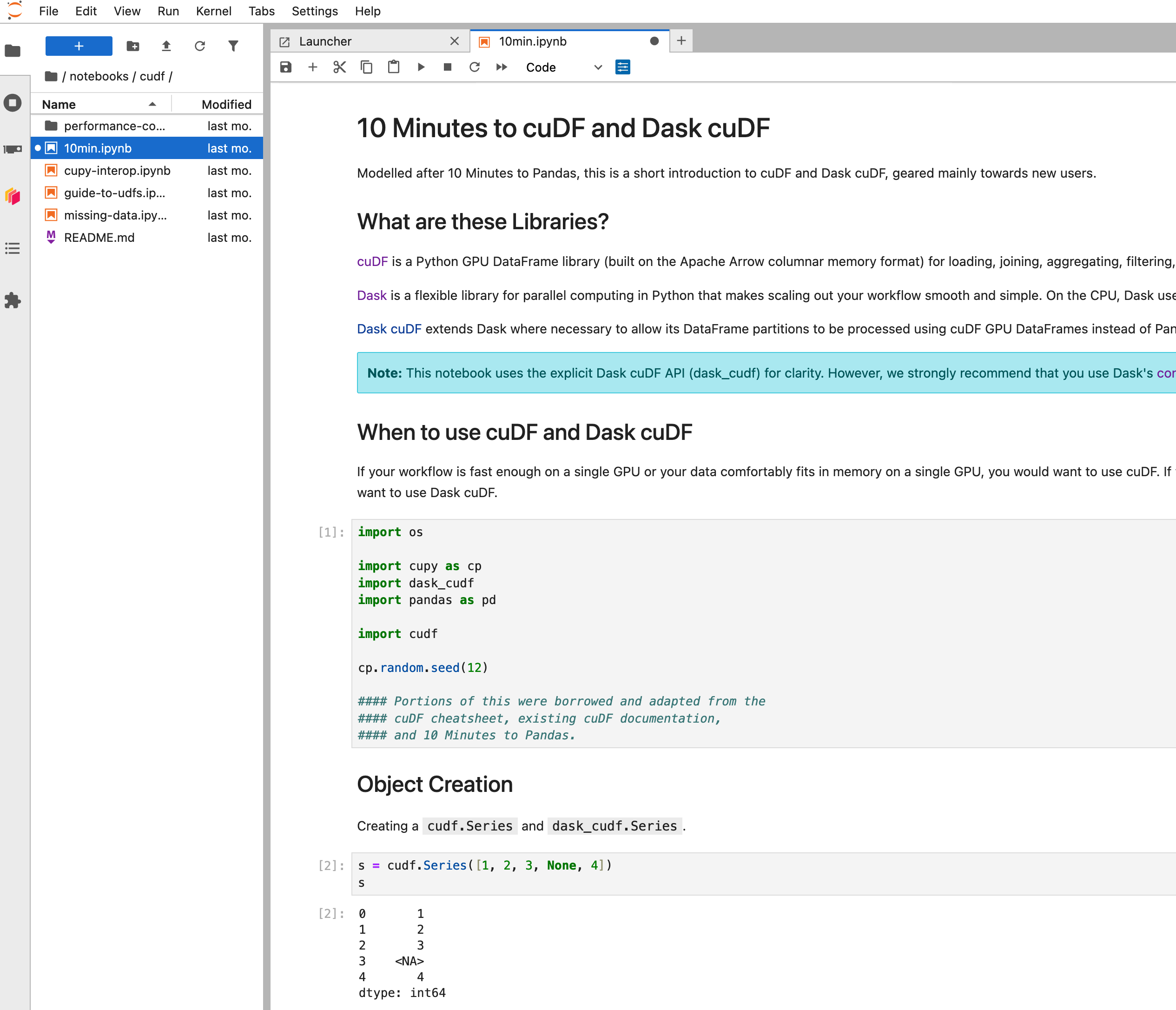
## Software Environments
By default when running remote operations Coiled will [attempt to create a copy of your local software environment](https://docs.coiled.io/user_guide/software/sync.html) which can be loaded onto the remote VMs. While this is an excellent feature it’s likely that you do not have all of the GPU software libraries you wish to use installed locally. In this case we need to tell Coiled which software environment to use.
### Container images
All Coiled commands can be passed a container image to use. This container will be pulled onto the remote VM at launch time.
```bash
$ coiled notebook start --gpu --container rapidsai/notebooks:25.12a-cuda12-py3.13
```
This is often the most convenient way to try out existing software environments, but is often not the most performant due to the way container images are unpacked.
### Coiled Software Environments
You can also created Coiled software environments ahead of time. These environments are built and cached on the cloud and can be pulled onto new VMs very quickly.
You can create a RAPIDS software environment using a conda `environment.yaml` file or a pip `requirements.txt` file.
#### Conda example
Create an environment file containing the RAPIDS packages
```yaml
# rapids-environment.yaml
name: rapidsai-notebooks
channels:
- { { rapids_conda_channel } }
- conda-forge
- nvidia
dependencies:
# RAPIDS packages
- rapids=25.12
- python=3.12
- cuda-version>=12.0,<=12.9
# (optional) Jupyter packages, necessary for Coiled Notebooks and Dask clusters with Jupyter enabled
- jupyterlab
- jupyterlab-nvdashboard
- dask-labextension
```
```bash
$ coiled env create --name rapids --gpu-enabled --conda rapids-environment.yaml
```
Then you can specify this software environment when starting new Coiled resources.
```bash
$ coiled notebook start --gpu --software rapidsai-notebooks
```
## CLI Jobs
You can execute a script in a container on an ephemeral VM with [Coiled CLI Jobs](https://docs.coiled.io/user_guide/cli-jobs.html).
```bash
$ coiled run python my_code.py # Boots a VM on the cloud, runs the scripts, then shuts down again
```
We can use this to run GPU code on a remote environment using the RAPIDS container. You can set the coiled CLI to keep the VM around for a few minutes after execution is complete just in case you want to run it again and reuse the same hardware.
```bash
$ coiled run --gpu --name rapids-demo --keepalive 5m --container rapidsai/base:25.12a-cuda12-py3.13 -- python my_code.py
...
```
This works very nicely when paired with the cudf.pandas CLI tool. For example we can run `python -m cudf.pandas my_script` to GPU accelerate our Pandas code without having to rewrite anything. For example [this script](https://gist.github.com/jacobtomlinson/2481ecf2e1d2787ae2864a6712eef97b#file-cudf_pandas_coiled_demo-py) processes some open NYC parking data. With `pandas` it takes around a minute, but with `cudf.pandas` it only takes a few seconds.
```bash
$ coiled run --gpu --name rapids-demo --keepalive 5m --container rapidsai/base:25.12a-cuda12-py3.13 -- python -m cudf.pandas cudf_pandas_coiled_demo.py
Output
------
This container image and its contents are governed by the NVIDIA Deep Learning Container License.
By pulling and using the container, you accept the terms and conditions of this license:
https://developer.download.nvidia.com/licenses/NVIDIA_Deep_Learning_Container_License.pdf
Calculate violations by state took: 3.470 seconds
Calculate violations by vehicle type took: 0.145 seconds
Calculate violations by day of week took: 1.238 seconds
```
## Notebooks
To start an interactive Jupyter notebook session with [Coiled Notebooks](https://docs.coiled.io/user_guide/notebooks.html) run the RAPIDS notebook container via the notebook service.
```bash
$ coiled notebook start --gpu --container rapidsai/notebooks:25.12a-cuda12-py3.13
```
Note that the `--gpu` flag will automatically select a `g4dn.xlarge` instance with a T4 GPU on AWS. You could additionally add the `--vm-type` flag to explicitly choose another machine type with different GPU configuration. For example to choose a machine with 4 L4 GPUs you would run the following.
```bash
$ coiled notebook start --gpu --vm-type g6.24xlarge --container nvcr.io/nvidia/rapidsai/notebooks:24.12-cuda12.5-py3.12
```
## Dask Clusters
Coiled’s [managed Dask clusters](https://docs.coiled.io/user_guide/dask.html) can also provision clusters using [dask-cuda](https://docs.rapids.ai/api/dask-cuda/nightly/) to enable using RAPIDS in a distributed way.
```python
cluster = coiled.Cluster(
container="rapidsai/notebooks:25.12a-cuda12-py3.13", # specify the software env to use
jupyter=True, # run Jupyter server on scheduler
scheduler_gpu=True, # add GPU to scheduler
n_workers=4,
worker_gpu=1, # single T4 per worker
worker_class="dask_cuda.CUDAWorker", # recommended
)
```
Once the cluster has started you can also get the Jupyter URL and navigate to Jupyter Lab running on the Dask Scheduler node.
```python
>>> print(cluster.jupyter_link)
https://cluster-abc123.dask.host/jupyter/lab?token=dddeeefff444555666
```
We can run `!nvidia-smi` in our notebook to see information on the GPU available to Jupyter.
We can also connect a Dask client to see that information for the workers too.
```python
from dask.distributed import Client
client = Client()
client
```
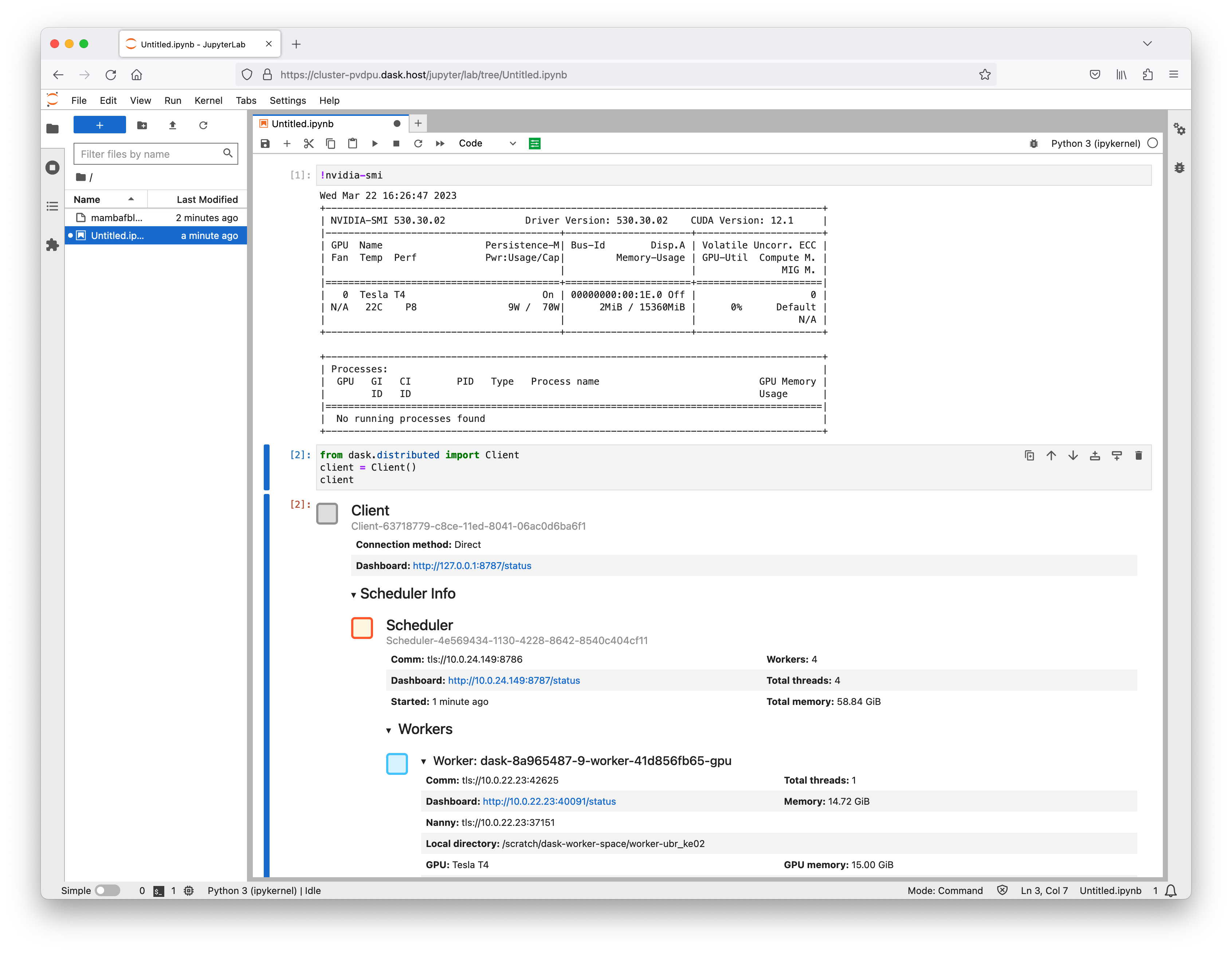
From this Jupyter session we can see that our notebook server has a GPU and we can connect to the Dask cluster with no configuration and see all the Dask Workers have GPUs too.
# index.html.md
# Kubeflow
You can use RAPIDS with Kubeflow in a single Pod with [Kubeflow Notebooks](https://www.kubeflow.org/docs/components/notebooks/) or you can scale out to many Pods on many nodes of the Kubernetes cluster with the [dask-operator](../tools/kubernetes/dask-operator.md).
#### NOTE
These instructions were tested against [Kubeflow v1.5.1](https://github.com/kubeflow/manifests/releases/tag/v1.5.1) running on [Kubernetes v1.21](https://kubernetes.io/blog/2021/04/08/kubernetes-1-21-release-announcement/). Visit [Installing Kubeflow](https://www.kubeflow.org/docs/started/installing-kubeflow/) for instructions on installing Kubeflow on your Kubernetes cluster.
## Kubeflow Notebooks
The [RAPIDS docker images](https://docs.rapids.ai/install/#docker) can be used directly in Kubeflow Notebooks with no additional configuration. To find the latest image head to [the RAPIDS install page](https://docs.rapids.ai/install), as shown in below, and choose a version of RAPIDS to use. Typically we want to choose the container image for the latest release. Verify the Docker image is selected when installing the latest RAPIDS release.
Be sure to match the CUDA version in the container image with that installed on your Kubernetes nodes. The default CUDA version installed on GKE Stable is 11.4 for example, so we would want to choose that. From 11.5 onwards it doesn’t matter as they will be backward compatible. Copy the container image name from the install command (i.e. `rapidsai/base:25.12a-cuda12-py3.13`).
#### NOTE
You can [check your CUDA version](https://jacobtomlinson.dev/posts/2022/how-to-check-your-nvidia-driver-and-cuda-version-in-kubernetes/) by creating a Pod and running `nvidia-smi`. For example:
```console
$ kubectl run nvidia-smi --restart=Never --rm -i --tty --image nvidia/cuda:11.0.3-base-ubuntu20.04 -- nvidia-smi
+-----------------------------------------------------------------------------+
| NVIDIA-SMI 495.46 Driver Version: 495.46 CUDA Version: 11.5 |
|-------------------------------+----------------------+----------------------+
...
```
Now in Kubeflow, access the Notebooks tab on the left and click “New Notebook”.

On this page, we must set a few configuration options. First, let’s give it a name like `rapids`. We need to check the “use custom image” box and paste in the container image we got from the RAPIDS release selector. Then, we want to set the CPU and RAM to something a little higher (i.e. 2 CPUs and 8GB memory) and set the number of NVIDIA GPUs to 1.

Then, you can scroll to the bottom of the page and hit launch. You should see it starting up in your list. The RAPIDS container images are packed full of amazing tools so this step can take a little while.

You can verify everything works okay by opening a terminal in Jupyter and running:
```bash
$ nvidia-smi
```

The RAPIDS container also comes with some example notebooks which you can find in `/rapids/notebooks`. You can make a symbolic link to these from your home directory so you can easily navigate using the file explorer on the left `ln -s /rapids/notebooks /home/jovyan/notebooks`.
Now you can navigate those example notebooks and explore all the libraries RAPIDS offers. For example, ETL developers that use [Pandas](https://pandas.pydata.org/) should check out the [cuDF](https://docs.rapids.ai/api/cudf/nightly/) notebooks for examples of accelerated dataframes.

## Scaling out to many GPUs
Many of the RAPIDS libraries also allow you to scale out your computations onto many GPUs spread over many nodes for additional acceleration. To do this we leverage [Dask](https://www.dask.org/), an open source Python library for distributed computing.
To use Dask, we need to create a scheduler and some workers that will perform our calculations. These workers will also need GPUs and the same Python environment as your notebook session. Dask has [an operator for Kubernetes](../tools/kubernetes/dask-operator.md) that you can use to manage Dask clusters on your Kubeflow cluster.
### Installing the Dask Kubernetes operator
To install the operator we need to create any custom resources and the operator itself, please [refer to the documentation](https://kubernetes.dask.org/en/latest/installing.html) to find up-to-date installation instructions. From the terminal run the following command.
```console
$ helm install --repo https://helm.dask.org --create-namespace -n dask-operator --generate-name dask-kubernetes-operator
NAME: dask-kubernetes-operator-1666875935
NAMESPACE: dask-operator
STATUS: deployed
REVISION: 1
TEST SUITE: None
NOTES:
Operator has been installed successfully.
```
Verify our resources were applied successfully by listing our Dask clusters. Don’t expect to see any resources yet but the command should succeed.
```console
$ kubectl get daskclusters
No resources found in default namespace.
```
You can also check the operator Pod is running and ready to launch new Dask clusters.
```console
$ kubectl get pods -A -l app.kubernetes.io/name=dask-kubernetes-operator
NAMESPACE NAME READY STATUS RESTARTS AGE
dask-operator dask-kubernetes-operator-775b8bbbd5-zdrf7 1/1 Running 0 74s
```
Lastly, ensure that your notebook session can create and manage Dask custom resources. To do this you need to edit the `kubeflow-kubernetes-edit` cluster role that gets applied to notebook Pods. Add a new rule to the rules section for this role to allow everything in the `kubernetes.dask.org` API group.
```console
$ kubectl edit clusterrole kubeflow-kubernetes-edit
…
rules:
…
- apiGroups:
- "kubernetes.dask.org"
verbs:
- "*"
resources:
- "*"
…
```
### Creating a Dask cluster
Now you can create `DaskCluster` resources in Kubernetes that will launch all the necessary Pods and services for our cluster to work. This can be done in YAML via the Kubernetes API or using the Python API from a notebook session as shown in this section.
In a Jupyter session, create a new notebook and install the `dask-kubernetes` package which you will need to launch Dask clusters.
```ipython
!pip install dask-kubernetes
```
Next, create a Dask cluster using the `KubeCluster` class. Set the container image to match the one used for your notebook environment and set the number of GPUs to 1. Also tell the RAPIDS container not to start Jupyter by default and run our Dask command instead.
This can take a similar amount of time to starting up the notebook container as it will also have to pull the RAPIDS docker image.
```python
from dask_kubernetes.experimental import KubeCluster
cluster = KubeCluster(
name="rapids-dask",
image="rapidsai/base:25.12a-cuda12-py3.13",
worker_command="dask-cuda-worker",
n_workers=2,
resources={"limits": {"nvidia.com/gpu": "1"}},
)
```

You can scale this cluster up and down either with the scaling tab in the widget in Jupyter or by calling `cluster.scale(n)` to set the number of workers (and therefore the number of GPUs).
Now you can connect a Dask client to our cluster and from that point on any RAPIDS libraries that support dask such as `dask_cudf` will use our cluster to distribute our computation over all of our GPUs.

## Accessing the Dask dashboard from notebooks
When working interactively in a notebook and leveraging a Dask cluster it can be really valuable to see the Dask dashboard. The dashboard is available on the scheduler `Pod` in the Dask cluster so we need to set some extra configuration to make this available from our notebook `Pod`.
To do this, we can apply the following manifest.
```yaml
# configure-dask-dashboard.yaml
apiVersion: "kubeflow.org/v1alpha1"
kind: PodDefault
metadata:
name: configure-dask-dashboard
spec:
selector:
matchLabels:
configure-dask-dashboard: "true"
desc: "configure dask dashboard"
env:
- name: DASK_DISTRIBUTED__DASHBOARD__LINK
value: "{NB_PREFIX}/proxy/{host}:{port}/status"
volumeMounts:
- name: jupyter-server-proxy-config
mountPath: /root/.jupyter/jupyter_server_config.py
subPath: jupyter_server_config.py
volumes:
- name: jupyter-server-proxy-config
configMap:
name: jupyter-server-proxy-config
---
apiVersion: v1
kind: ConfigMap
metadata:
name: jupyter-server-proxy-config
data:
jupyter_server_config.py: |
c.ServerProxy.host_allowlist = lambda app, host: True
```
Create a file with the above contents, and then apply it into your user’s namespace with `kubectl`.
For the default `user@example.com` user it would look like this.
```bash
$ kubectl apply -n kubeflow-user-example-com -f configure-dask-dashboard.yaml
```
This configuration file does two things. First it configures the [jupyter-server-proxy](https://github.com/jupyterhub/jupyter-server-proxy) running in your Notebook container to allow proxying to all hosts. We can do this safely because we are relying on Kubernetes (and specifically Istio) to enforce network access controls. It also sets the `distributed.dashboard-link` config option in Dask so that the widgets and `.dashboard_link` attributes of the `KubeCluster` and `Client` objects show a url that uses the Jupyter server proxy.
Once you have created this configuration option you can select it when launching new notebook instances.

You can then follow the links provided by the widgets in your notebook to open the Dask Dashboard in a new tab.

You can also use the [Dask Jupyter Lab extension](https://github.com/dask/dask-labextension) to view various plots and stats about your Dask cluster right in Jupyter Lab. Open up the Dask tab on the left side menu and click the little search icon, this will connect Jupyter lab to the dashboard via the client in your notebook. Then you can click the various plots you want to see and arrange them in Jupyter Lab however you like by dragging the tabs around.

### Related Examples
Scaling up Hyperparameter Optimization with Multi-GPU Workload on Kubernetes
library/xgboost
library/optuna
library/dask
library/dask-kubernetes
library/scikit-learn
workflow/hpo
dataset/nyc-taxi
data-storage/gcs
data-format/csv
platforms/kubeflow
platforms/kubernetes
Scaling up Hyperparameter Optimization with Kubernetes and XGBoost GPU Algorithm
library/xgboost
library/optuna
library/dask
tools/dask-kubernetes
library/scikit-learn
workflow/hpo
platforms/kubeflow
platforms/kubernetes
# index.html.md
# Continuous Integration
GitHub Actions
Run tests in GitHub Actions that depend on RAPIDS and NVIDIA GPUs.
single-node
# index.html.md
# Anaconda Cloud Notebooks
You can run RAPIDS workloads on [Anaconda Cloud Notebooks](https://www.anaconda.com/products/notebooks) by leveraging remote runtimes.
## Overview
To get started, sign up for an Anaconda account and choose the [Starter Tier](https://www.anaconda.com/pricing).
Navigate to [nb.anaconda.com](https://nb.anaconda.com/) and start your server.
Once logged into JupyterLab, open the launcher and select “Launch a Remote Runtime”.
Select an NVIDIA runtime.
Create a notebook and change the current runtime to your NVIDIA runtime.
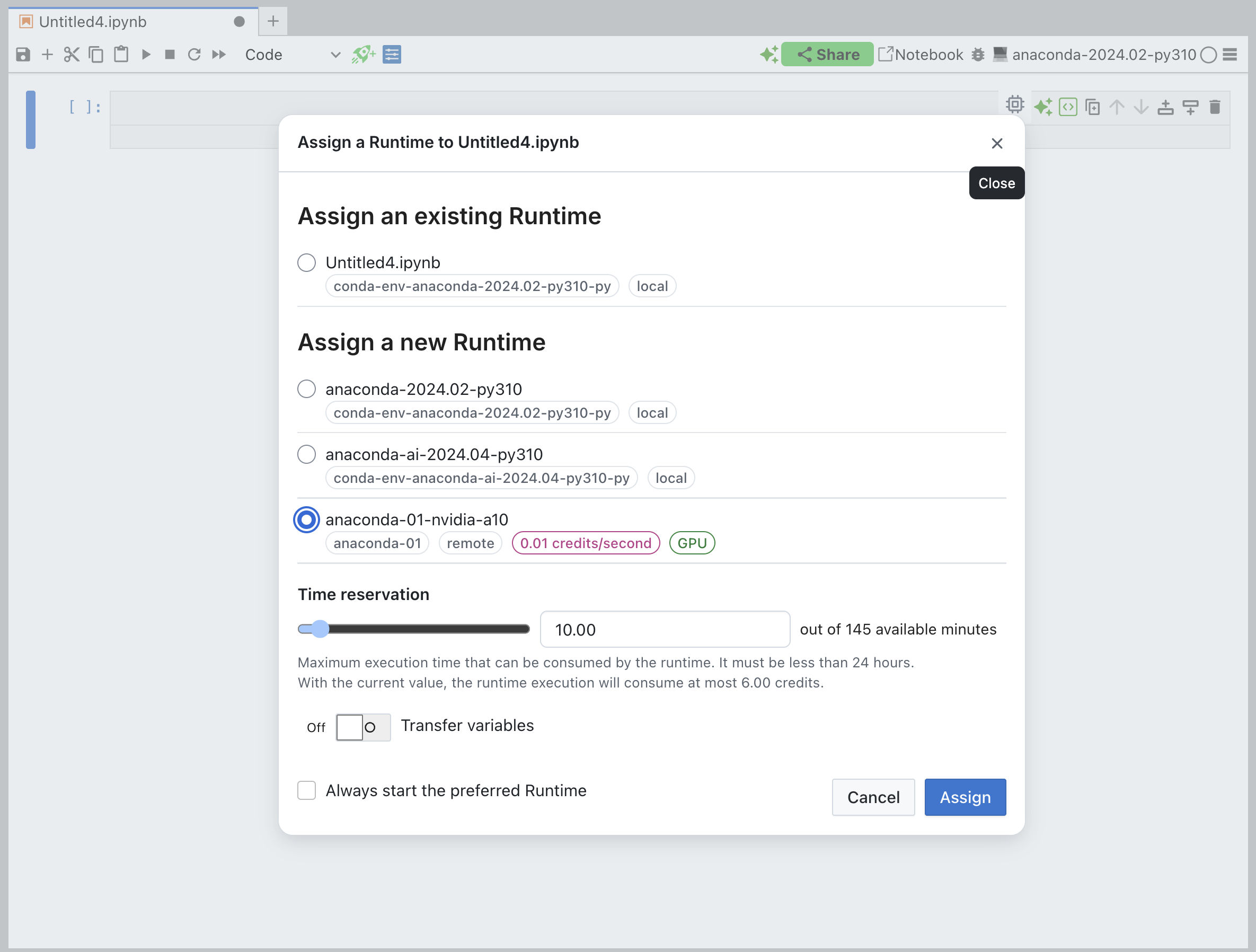
You will find common RAPIDS libraries including `cudf` and `cuml` already available in this environment and ready to use.
# index.html.md
# Snowflake
You can access `cuDF` and `cuML` in the [Snowflake Notebooks on Container Runtime for ML](https://docs.snowflake.com/en/developer-guide/snowflake-ml/notebooks-on-spcs).
Or you can install RAPIDS on [Snowflake](https://www.snowflake.com) via [Snowpark Container Services](https://docs.snowflake.com/en/developer-guide/snowpark-container-services/overview).
## Snowflake requirements
- A non-trial Snowflake account in AWS or Azure for Notebooks, and for container services an account in a
supported [AWS region](https://docs.snowflake.com/en/developer-guide/snowpark-container-services/overview#available-regions)
- A Snowflake account login with a role that has the `ACCOUNTADMIN` role. If not, you will need to work with your `ACCOUNTADMIN`
to perform the initial account setup.
- Access to `INSTANCE_FAMILY` with NVIDIA GPUs. For this guides we will use `GPU_NV_S` (1 NVIDIA A10G - smallest NVIDIA GPU size
available for Snowpark Containers to get started, and smallest instance type available for Notebooks)
## `cuDF` and `cuML` in Snowflake Notebooks ML Runtime
The [Snowflake Notebooks on Container Runtime for ML](https://docs.snowflake.com/en/developer-guide/snowflake-ml/notebooks-on-spcs)
has `cuDF` and `cuML` built in in the environment. If you want more control over your environment, or a closer experience to a Jupyter
Notebook setup, follow the instructions for [RAPIDS on Snowflake via Snowpark Container Services](#rapids-snowpark)
#### NOTE
The following instructions are an adaptation of the [Getting Started with Snowflake Notebook Container Runtime](https://quickstarts.snowflake.com/guide/notebook-container-runtime/#1)
and the [Train an XGBoost Model with GPUs using Snowflake Notebooks](https://quickstarts.snowflake.com/guide/train-an-xgboost-model-with-gpus-using-snowflake-notebooks/#1) guides from the Snowflake documentation.
### Set up the Snowflake Notebooks
In a SQL worksheet in Snowflake, run the following commands to create all the necessary requirements
to get started:
```sql
USE ROLE accountadmin;
CREATE OR REPLACE DATABASE container_runtime_lab;
CREATE SCHEMA notebooks;
CREATE OR REPLACE ROLE container_runtime_lab_user;
GRANT ROLE container_runtime_lab_user to USER naty;
GRANT USAGE ON DATABASE container_runtime_lab TO ROLE container_runtime_lab_user;
GRANT ALL ON SCHEMA container_runtime_lab.notebooks TO ROLE container_runtime_lab_user;
GRANT CREATE STAGE ON SCHEMA container_runtime_lab.notebooks TO ROLE container_runtime_lab_user;
GRANT CREATE NOTEBOOK ON SCHEMA container_runtime_lab.notebooks TO ROLE container_runtime_lab_user;
GRANT CREATE SERVICE ON SCHEMA container_runtime_lab.notebooks TO ROLE container_runtime_lab_user;
CREATE OR REPLACE WAREHOUSE CONTAINER_RUNTIME_WH AUTO_SUSPEND = 60;
GRANT ALL ON WAREHOUSE CONTAINER_RUNTIME_WH TO ROLE container_runtime_lab_user;
-- Create and grant access to EAIs
-- Create network rules (these are schema-level objects; end users do not need direct access to the network rules)
create network rule allow_all_rule
TYPE = 'HOST_PORT'
MODE= 'EGRESS'
VALUE_LIST = ('0.0.0.0:443','0.0.0.0:80');
-- Create external access integration (these are account-level objects; end users need access to this to access
-- the public internet with endpoints defined in network rules)
-- If you need to restrict access and create a different network rule, check pypi_network_rule example in
-- https://quickstarts.snowflake.com/guide/notebook-container-runtime/#1
CREATE OR REPLACE EXTERNAL ACCESS INTEGRATION allow_all_integration
ALLOWED_NETWORK_RULES = (allow_all_rule)
ENABLED = true;
GRANT USAGE ON INTEGRATION allow_all_integration TO ROLE container_runtime_lab_user;
-- Create compute pool to leverage multiple GPUs (see docs - https://docs.snowflake.com/en/developer-guide/snowpark-container-services/working-with-compute-pool)
CREATE COMPUTE POOL IF NOT EXISTS GPU_NV_S_compute_pool
MIN_NODES = 1
MAX_NODES = 1
INSTANCE_FAMILY = GPU_NV_S;
-- Grant usage of compute pool to newly created role
GRANT USAGE ON COMPUTE POOL GPU_NV_S_compute_pool to ROLE container_runtime_lab_user;
```
### Create or Upload a new Notebook
1. Make sure under your user you select the role `container_runtime_lab_user` that you just created during the setup step.

1. In the Snowflake app, on the left panel, go to **Projects** -> **Notebooks**. Once there you’ll be able to create a new
notebook by selecting the `+ Notebook` button, or if you click the dropdown you’ll be able to import one. In either case, you
will need to make some selections, make sure you select the right database, runtime version, compute pool, etc.

1. For this example we suggest you upload the following [notebook cuml example](https://github.com/rapidsai/deployment/tree/main/source/examples/cuml-snowflake-nb/notebook.ipynb).
2. Once the notebook is uploaded, we need to make sure we have access to the internet before we can get started. Go to
the three dots at the top right of your Snowflake app and select **Network settings**, then go to **External access**
and toggle on the network access `ALLOW_ALL_INTEGRATION` we created in the setup step, and hit **Save**

1. On the top right hit **Start** to get the compute pool going. After a few minutes you will see the status is **Active**,
run the notebook to see `cuml.accel` in action.
2. When you are done, end your session and suspend the compute pool.
## RAPIDS on Snowflake via Snowpark Container Services
#### NOTE
The following instructions are an adaptation of the [Introduction to Snowpark
container Services](https://quickstarts.snowflake.com/guide/intro_to_snowpark_container_services/#0) guide from the Snowflake documentation.
### Set up the Snowflake environment
In a SQL worksheet in Snowflake, run the following commands to create the role,
database, warehouse, and stage that we need to get started:
```sql
-- Create an CONTAINER_USER_ROLE with required privileges
USE ROLE ACCOUNTADMIN;
CREATE ROLE CONTAINER_USER_ROLE;
GRANT CREATE DATABASE ON ACCOUNT TO ROLE CONTAINER_USER_ROLE;
GRANT CREATE WAREHOUSE ON ACCOUNT TO ROLE CONTAINER_USER_ROLE;
GRANT CREATE COMPUTE POOL ON ACCOUNT TO ROLE CONTAINER_USER_ROLE;
GRANT CREATE INTEGRATION ON ACCOUNT TO ROLE CONTAINER_USER_ROLE;
GRANT MONITOR USAGE ON ACCOUNT TO ROLE CONTAINER_USER_ROLE;
GRANT BIND SERVICE ENDPOINT ON ACCOUNT TO ROLE CONTAINER_USER_ROLE;
GRANT IMPORTED PRIVILEGES ON DATABASE snowflake TO ROLE CONTAINER_USER_ROLE;
-- Grant CONTAINER_USER_ROLE to ACCOUNTADMIN
grant role CONTAINER_USER_ROLE to role ACCOUNTADMIN;
-- Create Database, Warehouse, and Image spec stage
USE ROLE CONTAINER_USER_ROLE;
CREATE OR REPLACE DATABASE CONTAINER_HOL_DB;
CREATE OR REPLACE WAREHOUSE CONTAINER_HOL_WH
WAREHOUSE_SIZE = XSMALL
AUTO_SUSPEND = 120
AUTO_RESUME = TRUE;
CREATE STAGE IF NOT EXISTS specs
ENCRYPTION = (TYPE='SNOWFLAKE_SSE');
CREATE STAGE IF NOT EXISTS volumes
ENCRYPTION = (TYPE='SNOWFLAKE_SSE')
DIRECTORY = (ENABLE = TRUE);
```
Then we proceed to create the external access integration, the compute pool (with
GPU resources), and the image repository:
```sql
USE ROLE ACCOUNTADMIN;
CREATE OR REPLACE NETWORK RULE ALLOW_ALL_RULE
TYPE = 'HOST_PORT'
MODE = 'EGRESS'
VALUE_LIST= ('0.0.0.0:443', '0.0.0.0:80');
CREATE OR REPLACE EXTERNAL ACCESS INTEGRATION ALLOW_ALL_EAI
ALLOWED_NETWORK_RULES = (ALLOW_ALL_RULE)
ENABLED = true;
GRANT USAGE ON INTEGRATION ALLOW_ALL_EAI TO ROLE CONTAINER_USER_ROLE;
USE ROLE CONTAINER_USER_ROLE;
CREATE COMPUTE POOL IF NOT EXISTS CONTAINER_HOL_POOL
MIN_NODES = 1
MAX_NODES = 1
INSTANCE_FAMILY = GPU_NV_S; -- instance with GPU
CREATE IMAGE REPOSITORY CONTAINER_HOL_DB.PUBLIC.IMAGE_REPO;
SHOW IMAGE REPOSITORIES IN SCHEMA CONTAINER_HOL_DB.PUBLIC;
```
### Docker image push via SnowCLI
The next step in the process is to push to the image registry the docker image
you will want to run via the service.
#### Build Docker image locally
For this guide, we build an image that starts from the RAPIDS notebook image and
adds some extra snowflake packages.
Create a Dockerfile as follow:
```Dockerfile
FROM rapidsai/notebooks:25.12a-cuda12-py3.13
RUN pip install "snowflake-snowpark-python[pandas]" snowflake-connector-python
```
#### NOTE
- The `python=3.11`, is the latest supported by the Snowflake connector package.
- The use of `amd64` platform is required by Snowflake.
Build the image in the directory where your Dockerfile is located. Notice that
no GPU is needed to build this image.
```bash
$ docker build --platform=linux/amd64 -t /rapids-nb-snowflake:latest .
```
#### Install SnowCLI
Install the SnowCLI following your preferred method instructions in the
[documentation](https://docs.snowflake.com/en/developer-guide/snowflake-cli/installation/installation).
Once installed, configure your Snowflake CLI connection, and follow the wizard:
#### NOTE
When you follow the wizard you will need `-`, you can obtain
them by running the following in the Snowflake SQL worksheet.
```sql
SELECT CURRENT_ORGANIZATION_NAME(); --org
SELECT CURRENT_ACCOUNT_NAME(); --account name
```
```bash
$ snow connection add
```
```bash
connection name : CONTAINER_HOL
account : - # e.g. MYORGANIZATION-MYACCOUNT
user :
password :
role: CONTAINER_USER_ROLE
warehouse : CONTAINER_HOL_WH
database : CONTAINER_HOL_DB
schema : public
host:
port:
region:
authenticator: username_password_mfa # only needed if MFA and MFA caching are enabled
private key file:
token file path:
```
Test the connection:
```bash
$ snow connection test --connection "CONTAINER_HOL"
```
To be able to push the docker image we need to get the snowflake registry hostname
from the repository url. In a Snowflake SQL worksheet run:
```sql
USE ROLE CONTAINER_USER_ROLE;
SHOW IMAGE REPOSITORIES IN SCHEMA CONTAINER_HOL_DB.PUBLIC;
```
You will see that the repository url is `org-account.registry.snowflakecomputing.com/container_hol_db/public/image_repo` where `org-account` refers to your organization and account, the `SNOWFLAKE_REGISTRY_HOSTNAME` is the url up to the `.com`. i.e. `org-account.registry.snowflakecomputing.com`
First we login into the snowflake image-registry via terminal:
#### NOTE
If you have **MFA** activated you will want to allow [client MFA caching] (https://docs.snowflake.com/en/user-guide/security-mfa#using-mfa-token-caching-to-minimize-the-number-of-prompts-during-authentication-optional)
to reduce the number of prompts that must be acknowledged while connecting and authenticating to Snowflake.
To enable this, you need `ACCOUNTADMIN` system role and in a sql sheet run:
```sql
ALTER ACCOUNT SET ALLOW_CLIENT_MFA_CACHING = TRUE;
```
and if you are using the Snowflake Connector for Python you need:
```bash
$ pip install "snowflake-connector-python[secure-local-storage]"
```
```bash
$ snow spcs image-registry login --connection CONTAINER_HOL
```
We tag and push the image, make sure you replace the repository url for `org-account.registry.snowflakecomputing.com/container_hol_db/public/image_repo`:
```bash
$ docker tag /rapids-nb-snowflake:latest /rapids-nb-snowflake:dev
```
Verify that the new tagged image exists by running:
```bash
$ docker image list
```
Push the image to snowflake:
```bash
$ docker push /rapids-nb-snowflake:dev
```
#### NOTE
This step will take some time, while this process completes we can continue
with next step to configure and push the Spec YAML.
When the `docker push` command completes, you can verify that the image exists in your Snowflake Image Repository by running the following in the Snowflake SQL worksheet
```sql
USE ROLE CONTAINER_USER_ROLE;
CALL SYSTEM$REGISTRY_LIST_IMAGES('/CONTAINER_HOL_DB/PUBLIC/IMAGE_REPO');
```
### Configure and Push Spec YAML
Snowpark Container Services are defined and configured using YAML files. There
is support for multiple parameters configurations, refer to then [Snowpark container services specification reference](https://docs.snowflake.com/en/developer-guide/snowpark-container-services/specification-reference) for more information.
Locally, create the following file `rapids-snowpark.yaml`:
```yaml
spec:
containers:
- name: rapids-nb-snowpark
image: .registry.snowflakecomputing.com/container_hol_db/public/image_repo/rapids-nb-snowflake:dev
volumeMounts:
- name: rapids-notebooks
mountPath: /home/rapids/notebooks/workspace
resources:
requests:
nvidia.com/gpu: 1
limits:
nvidia.com/gpu: 1
endpoints:
- name: jupyter
port: 8888
public: true
- name: dask-client
port: 8786
protocol: TCP
- name: dask-dashboard
port: 8787
public: true
volumes:
- name: rapids-notebooks
source: "@volumes/rapids-notebooks"
uid: 1001 # rapids user's UID
gid: 1000
```
Notice that in we mounted the `@volumes/rapids-notebooks` internal stage location
to our `/home/rapids/notebooks/workspace` directory inside of our running container.
Anything that is added to this directory will persist.
We use `snow-cli` to push this `yaml` file:
```bash
$ snow stage copy rapids-snowpark.yaml @specs --overwrite --connection CONTAINER_HOL
```
Verify that your `yaml` was pushed properly by running the following SQL in the
Snowflake worksheet:
```sql
USE ROLE CONTAINER_USER_ROLE;
LS @CONTAINER_HOL_DB.PUBLIC.SPECS;
```
### Create and Test the Service
Now that we have successfully pushed the image and the spec YAML, we have all
the components in Snowflake to create our service. We only need a service name,
a compute pool and the spec file. Run this SQL in the Snowflake worksheet:
```sql
USE ROLE CONTAINER_USER_ROLE;
CREATE SERVICE CONTAINER_HOL_DB.PUBLIC.rapids_snowpark_service
in compute pool CONTAINER_HOL_POOL
from @specs
specification_file='rapids-snowpark.yaml'
external_access_integrations = (ALLOW_ALL_EAI);
```
Run the following to verify that the service is successfully running.
```sql
CALL SYSTEM$GET_SERVICE_STATUS('CONTAINER_HOL_DB.PUBLIC.rapids_snowpark_service');
```
Since we specified the `jupyter` endpoint to be public, Snowflake will generate
a url that can be used to access the service via the browser. To get the url,
run in the SQL snowflake worksheet:
```sql
SHOW ENDPOINTS IN SERVICE RAPIDS_SNOWPARK_SERVICE;
```
Copy the jupyter `ingress_url` in the browser. You will see a jupyter lab with a set of
notebooks to get started with RAPIDS.

### Shutdown and Cleanup
If you no longer need the service and the compute pool up and running, we can
stop the service and suspend the compute pool to avoid incurring in any charges.
In the Snowflake SQL worksheet run:
```sql
USE ROLE CONTAINER_USER_ROLE;
ALTER COMPUTE POOL CONTAINER_HOL_POOL STOP ALL;
ALTER COMPUTE POOL CONTAINER_HOL_POOL SUSPEND;
```
If you want to cleanup completely and remove all of the objects created, run the
following:
```sql
USE ROLE CONTAINER_USER_ROLE;
ALTER COMPUTE POOL CONTAINER_HOL_POOL STOP ALL;
ALTER COMPUTE POOL CONTAINER_HOL_POOL SUSPEND;
DROP COMPUTE POOL CONTAINER_HOL_POOL;
DROP DATABASE CONTAINER_HOL_DB;
DROP WAREHOUSE CONTAINER_HOL_WH;
USE ROLE ACCOUNTADMIN;
DROP ROLE CONTAINER_USER_ROLE;
DROP EXTERNAL ACCESS INTEGRATION ALLOW_ALL_EAI;
```
#### Related Examples
Getting Started with cuML’s accelerator mode (cuml.accel) in Snowflake Notebooks
library/cuml
platforms/snowflake
Getting Started with cudf.pandas and Snowflake
library/cudf
platforms/snowflake
# index.html.md
# Databricks
You can install RAPIDS on Databricks in a few different ways:
1. Accelerate machine learning workflows in a single-node GPU notebook environment
2. Spark users can install [RAPIDS Accelerator for Apache Spark 3.x on Databricks](https://docs.nvidia.com/spark-rapids/user-guide/latest/getting-started/databricks.html)
3. Install Dask alongside Spark and then use libraries like `dask-cudf` for multi-node workloads
## Single-node GPU Notebook environment
### Create init-script
To get started, you must first configure an [initialization script](https://docs.databricks.com/en/init-scripts/index.html) to install RAPIDS libraries and all other dependencies for your project.
Databricks recommends using [cluster-scoped](https://docs.databricks.com/en/init-scripts/cluster-scoped.html) init scripts stored in the workspace files.
Navigate to the top-left **Workspace** tab and click on your **Home** directory then select **Add** > **File** from the menu. Create an `init.sh` script with contents:
```bash
#!/bin/bash
set -e
# Install RAPIDS libraries
pip install \
--extra-index-url=https://pypi.anaconda.org/rapidsai-wheels-nightly/simple \
"cudf-cu12>=25.12.*,>=0.0.0a0" "cuml-cu12>=25.12.*,>=0.0.0a0" \
"dask-cuda>=25.12.*,>=0.0.0a0"
```
### Launch cluster
To get started, navigate to the **All Purpose Compute** tab of the **Compute** section in Databricks and select **Create Compute**. Name your cluster and choose **“Single node”**.

In order to launch a GPU node uncheck **Use Photon Acceleration** and select any `15.x`, `16.x` or `17.x` ML LTS runtime with GPU support.
For example for long-term support releases you could select the `15.4 LTS ML (includes Apache Spark 3.5.0, GPU, Scala 2.12)` runtime version.
The “GPU accelerated” nodes should now be available in the **Node type** dropdown.

Then expand the **Advanced Options** section, open the **Init Scripts** tab and enter the file path to the init-script in your Workspace directory starting with `/Users//.sh` and click **“Add”**.

Select **Create Compute**
### Test RAPIDS
Once your cluster has started, you can create a new notebook or open an existing one from the `/Workspace` directory then attach it to your running cluster.
```python
import cudf
gdf = cudf.DataFrame({"a":[1,2,3],"b":[4,5,6]})
gdf
a b
0 1 4
1 2 5
2 3 6
```
#### Quickstart with cuDF Pandas
RAPIDS recently introduced cuDF’s [pandas accelerator mode](https://rapids.ai/cudf-pandas/) to accelerate existing pandas workflows with zero changes to code.
Using `cudf.pandas` in Databricks on a single-node can offer significant performance improvements over traditional pandas when dealing with large datasets; operations are optimized to run on the GPU (cuDF) whenever possible, seamlessly falling back to the CPU (pandas) when necessary, with synchronization happening in the background.
Below is a quick example how to load the `cudf.pandas` extension in a Jupyter notebook:
```python
%load_ext cudf.pandas
%%time
import pandas as pd
df = pd.read_parquet(
"nyc_parking_violations_2022.parquet",
columns=["Registration State", "Violation Description", "Vehicle Body Type", "Issue Date", "Summons Number"]
)
(df[["Registration State", "Violation Description"]]
.value_counts()
.groupby("Registration State")
.head(1)
.sort_index()
.reset_index()
)
```
Upload the [10 Minutes to RAPIDS cuDF Pandas notebook](https://colab.research.google.com/drive/12tCzP94zFG2BRduACucn5Q_OcX1TUKY3) in your single-node Databricks cluster and run through the cells.
**NOTE**: cuDF pandas is open beta and under active development. You can [learn more through the documentation](https://docs.rapids.ai/api/cudf/nightly/?_gl=1*1oyfbsi*_ga*MTc5NDYzNzYyNC4xNjgzMDc2ODc2*_ga_RKXFW6CM42*MTcwNTU4NDUyNS4yMC4wLjE3MDU1ODQ1MjUuNjAuMC4w) and the [release blog](https://developer.nvidia.com/blog/rapids-cudf-accelerates-pandas-nearly-150x-with-zero-code-changes/).
# index.html.md
# NVIDIA AI Workbench
[NVIDIA AI Workbench](https://www.nvidia.com/en-us/deep-learning-ai/solutions/data-science/workbench/) is a developer toolkit for data science, machine learning, and AI projects. It lets you develop on your laptop/workstation and then easily transition workloads to scalable GPU resources in a data center or the cloud. AI Workbench is free, you can install it in minutes on both local or remote computers, and offers a desktop application as well as a command-line interface (CLI).
## Installation
You can install AI Workbench locally, or on a remote computer that you have SSH access to.
Follow the [AI Workbench installation](https://docs.nvidia.com/ai-workbench/user-guide/latest/installation/overview.html) documentation for instructions on installing on different operating systems.
## Configure your system
Once you have installed AI Workbench you can launch the desktop application. On first run it will talk you through installing some dependencies if they aren’t available already.
Then you will be able to choose between using your local environment or working on a remote system (you can switch between them later very easily).
If you wish to configure a remote system click the “Add Remote System” button and enter the configuration information for that system.
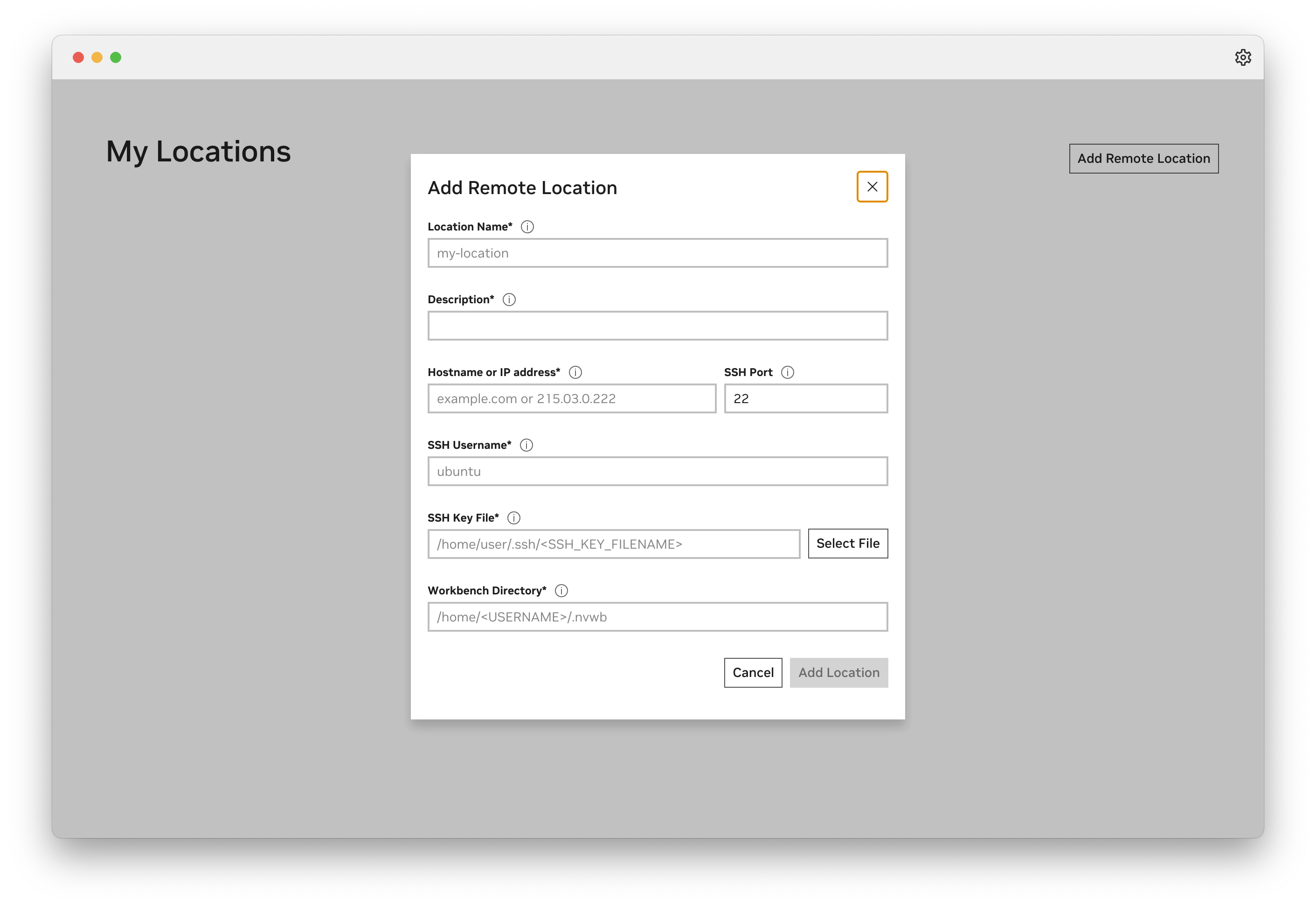
Once configured select the system you wish to use. You will then be greeted with a screen where you can create a new project or clone an existing one.
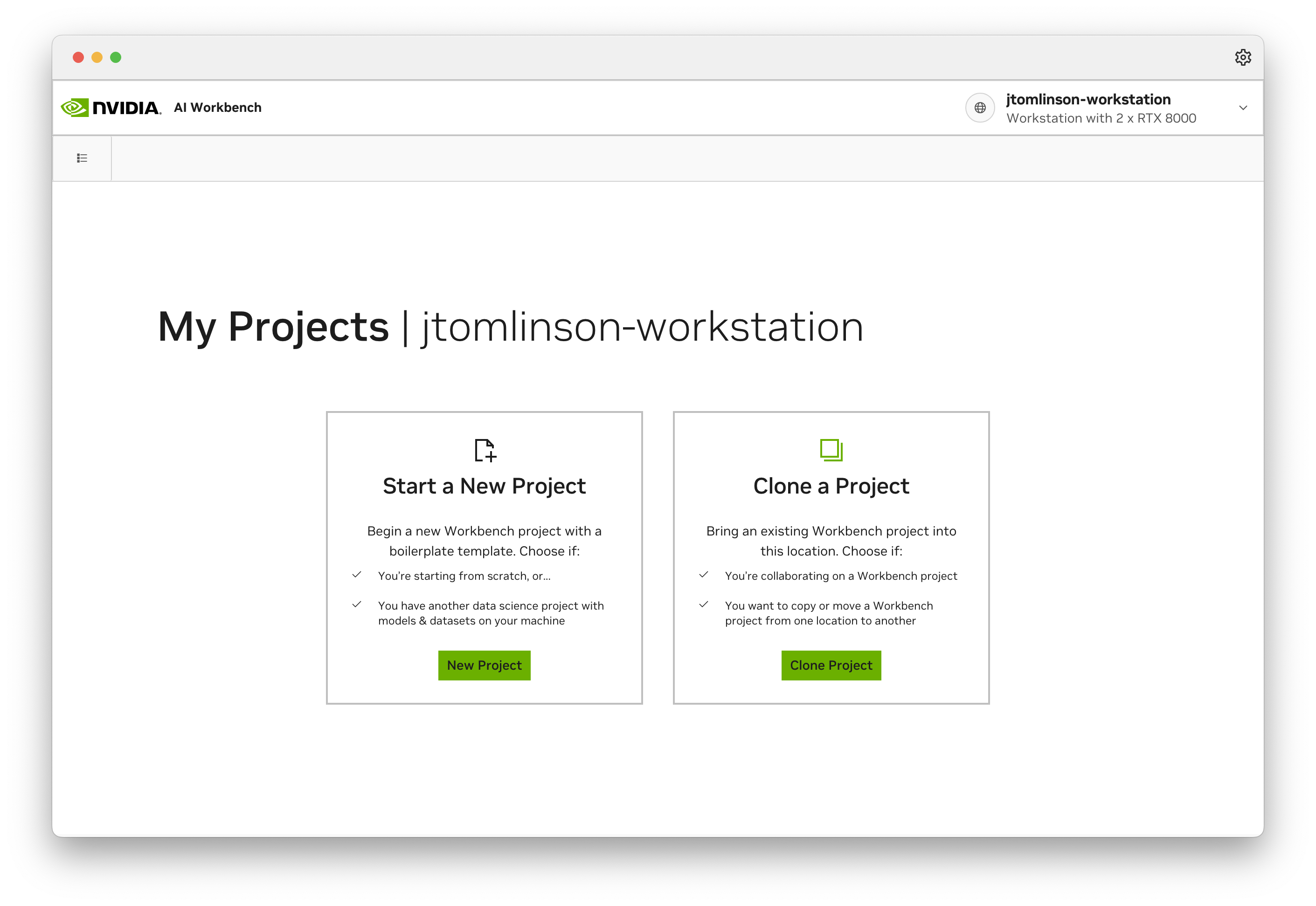
Select “Start a new project” and give it a name and description. You can also change the default location to store the project files.
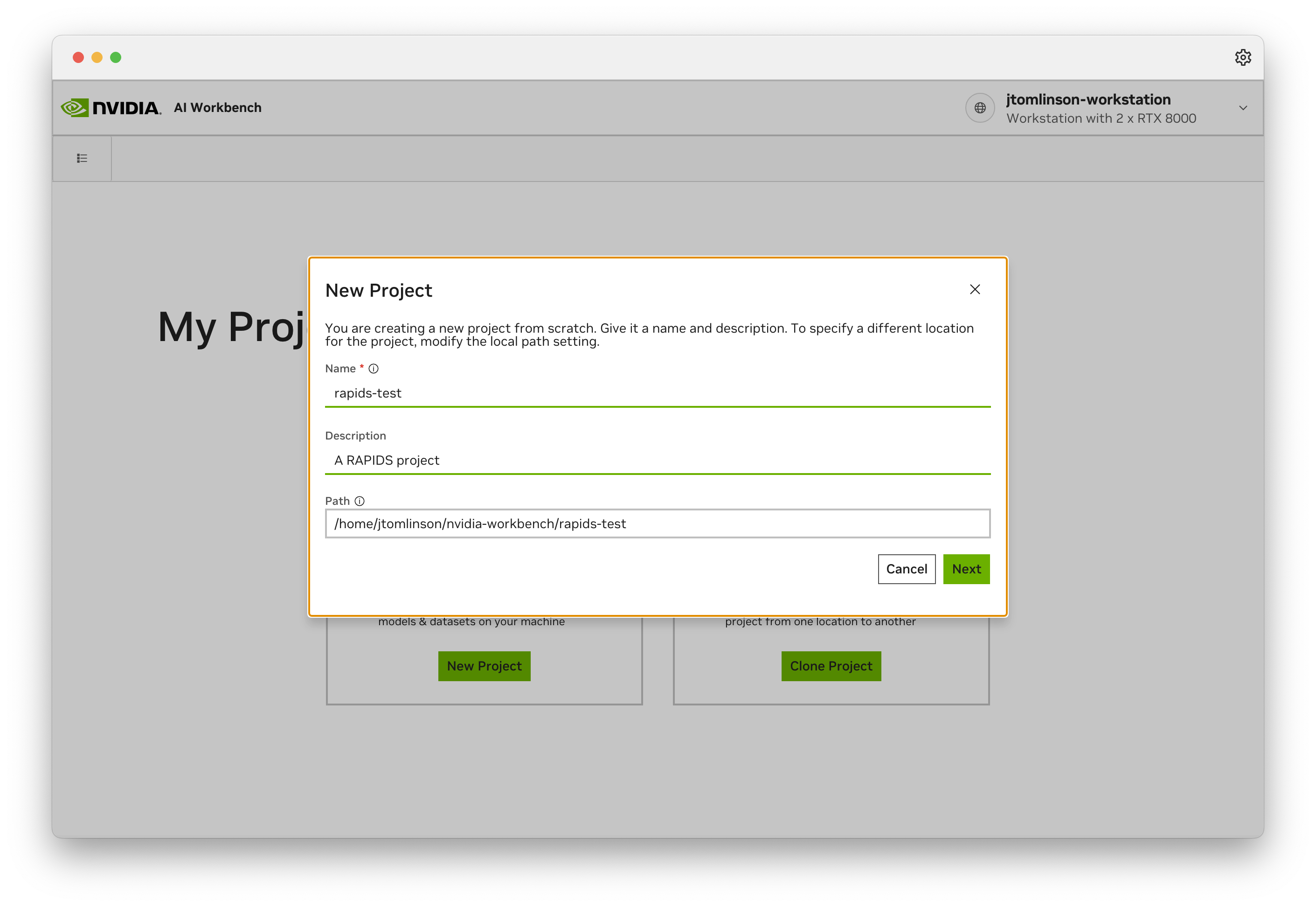
Then scroll down and select “RAPIDS with CUDA” from the list of templates.
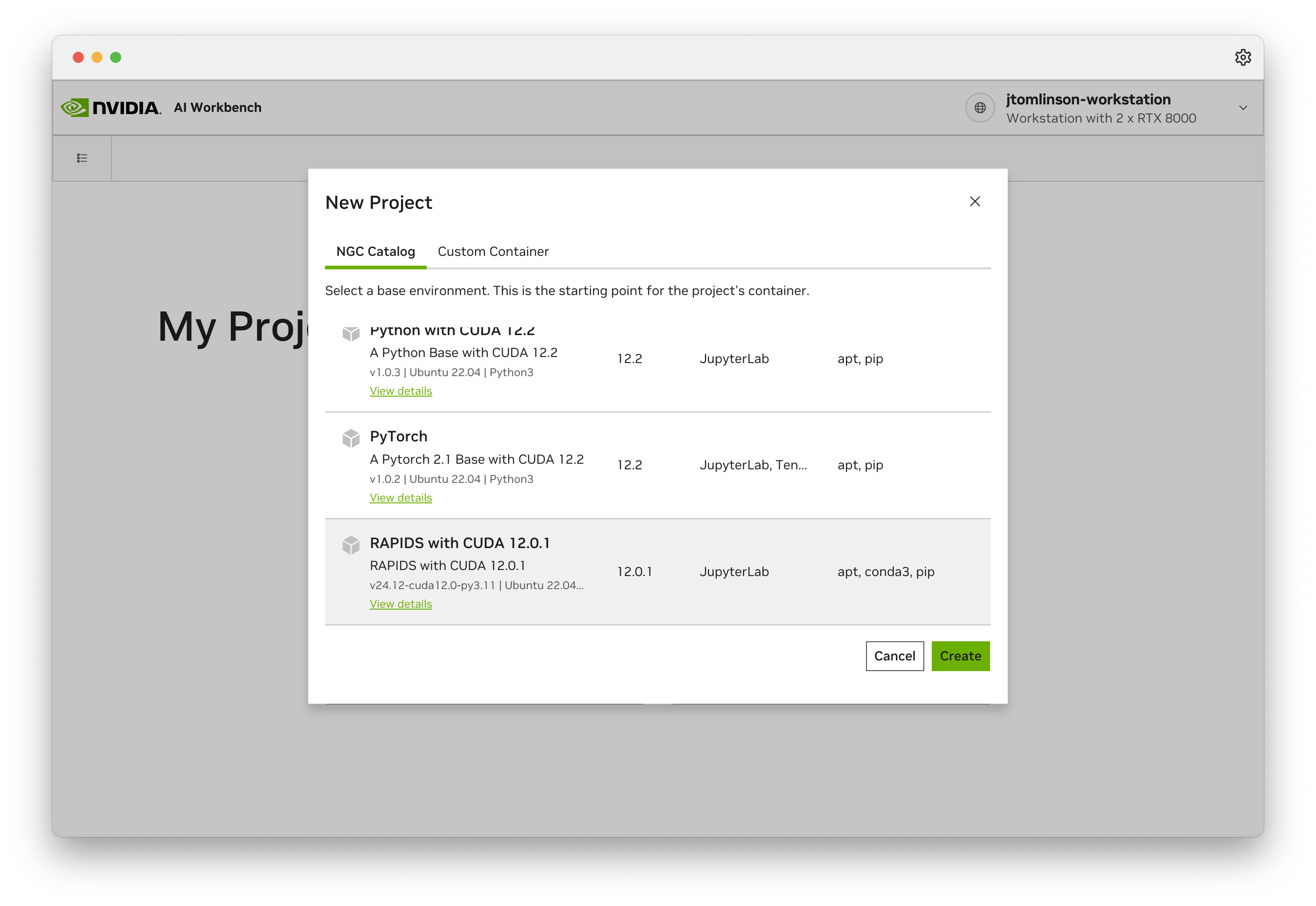
The new project will then be created. AI Workbench will automatically build a container for this project, this may take a few minutes.
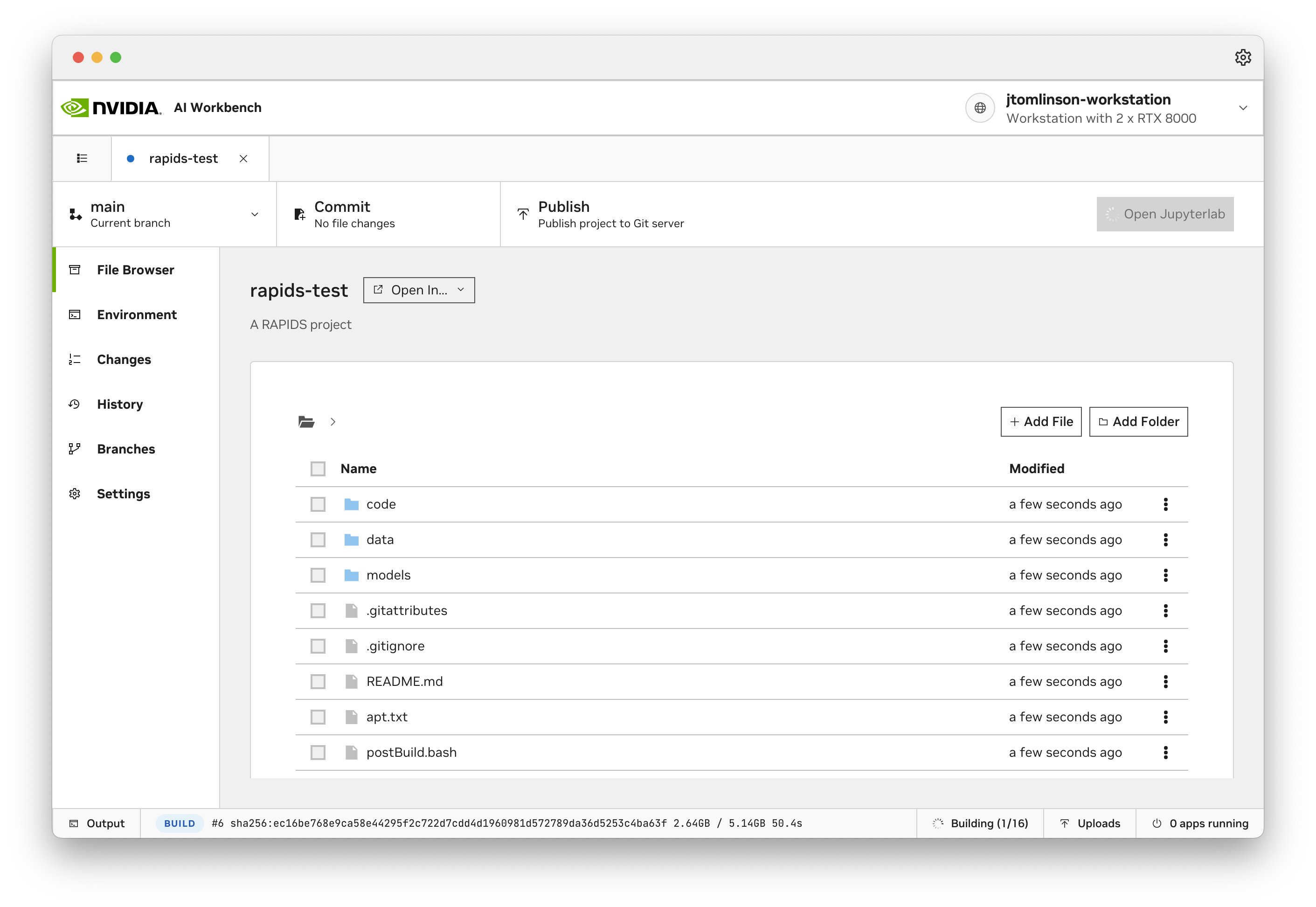
Once the project has built you can select “Open Jupyterlab” to launch Jupyter in your RAPIDS environment.
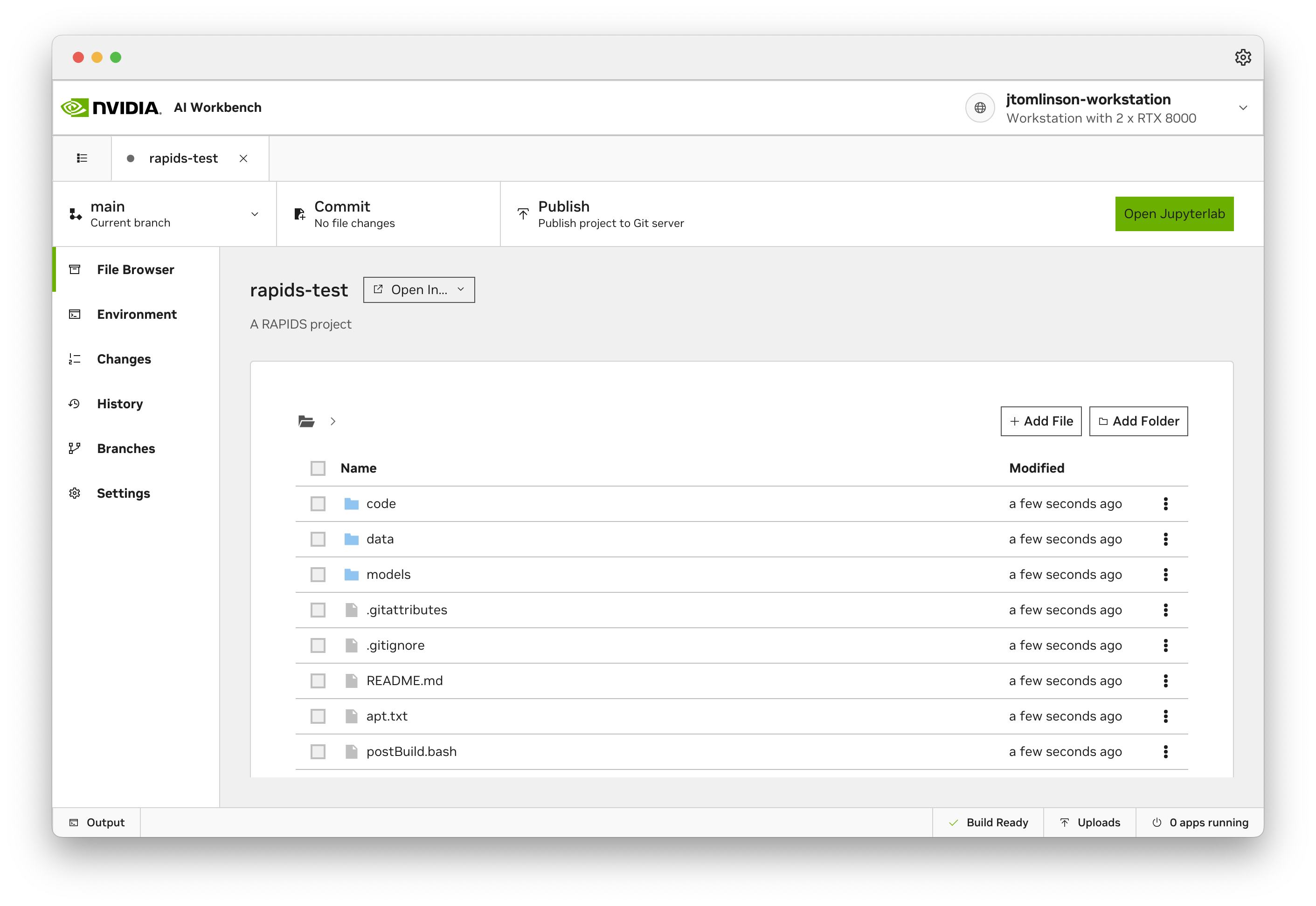
Then you can start working with the RAPIDS libraries in your notebooks.
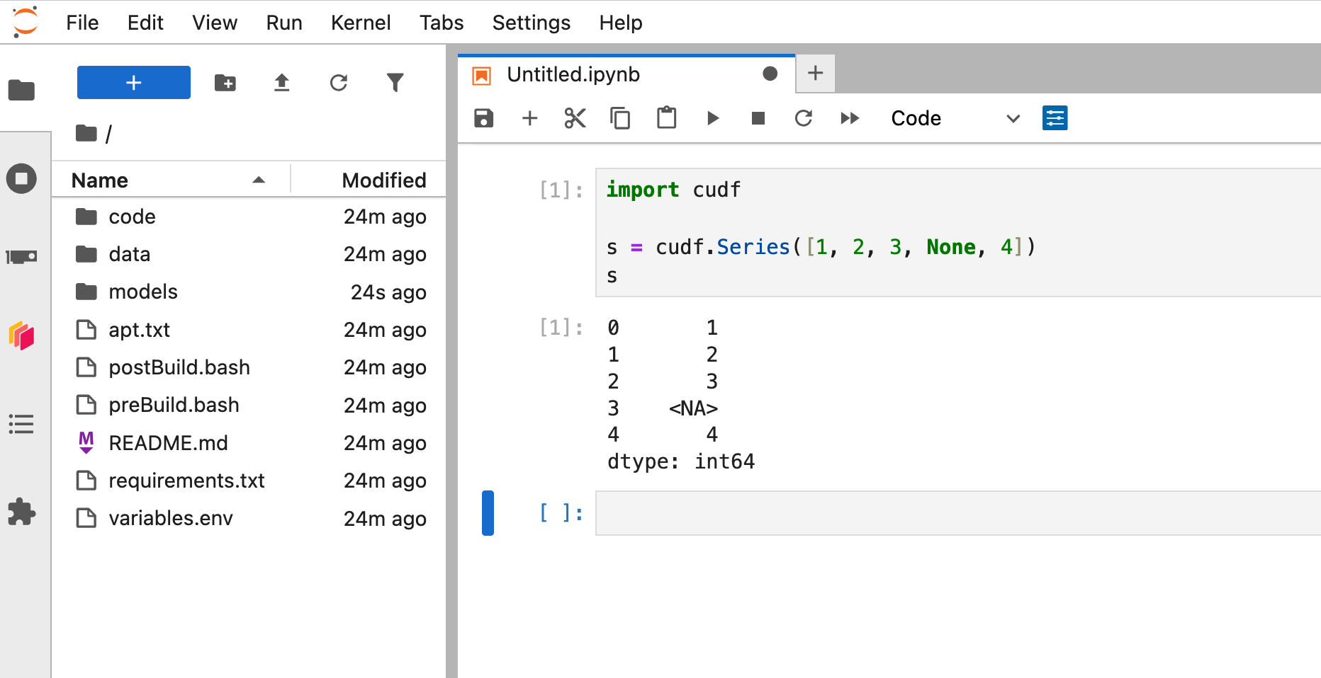
## Further reading
For more information and to learn more about what you can do with NVIDIA AI Workbench [see the documentation](https://docs.nvidia.com/ai-workbench/user-guide/latest/overview/introduction.html).
# index.html.md
# KServe
[KServe](https://kserve.github.io/website) is a standard model inference platform built for Kubernetes. It provides consistent interface for multiple machine learning frameworks.
In this page, we will show you how to deploy RAPIDS models using KServe.
#### NOTE
These instructions were tested against KServe v0.10 running on [Kubernetes v1.21](https://kubernetes.io/blog/2021/04/08/kubernetes-1-21-release-announcement/).
## Setting up Kubernetes cluster with GPU access
First, you should set up a Kubernetes cluster with access to NVIDIA GPUs. Visit [the Cloud Section](../cloud/index.md) for guidance.
## Installing KServe
Visit [Getting Started with KServe](https://kserve.github.io/website/latest/get_started/) to install KServe in your Kubernetes cluster. If you are starting out, we recommend the use of the “Quickstart” script (`quick_install.sh`) provided in the page. On the other hand, if you are setting up a production-grade system, follow direction in [Administration Guide](https://kserve.github.io/website/latest/admin/serverless/serverless) instead.
## Setting up First InferenceService
Once KServe is installed, visit [First InferenceService](https://kserve.github.io/website/latest/get_started/first_isvc/) to quickly set up a first inference endpoint. (The example uses the [Support Vector Machine from scikit-learn](https://scikit-learn.org/stable/modules/generated/sklearn.svm.SVC.html) to classify [the Iris dataset](https://scikit-learn.org/stable/auto_examples/datasets/plot_iris_dataset.html).) Follow through all the steps carefully and make sure everything works. In particular, you should be able to submit inference requests using cURL.
## Setting up InferenceService with Triton-FIL
[The FIL backend for Triton Inference Server](https://github.com/triton-inference-server/fil_backend) (Triton-FIL in short) is an optimized inference runtime for many kinds of tree-based models including: XGBoost, LightGBM, scikit-learn, and cuML RandomForest. We can use Triton-FIL together with KServe and serve any tree-based models.
The following manifest sets up an inference endpoint using Triton-FIL:
```yaml
# triton-fil.yaml
apiVersion: serving.kserve.io/v1beta1
kind: InferenceService
metadata:
name: triton-fil
spec:
predictor:
triton:
storageUri: gs://path-to-gcloud-storage-bucket/model-directory
runtimeVersion: 22.12-py3
```
where `model-directory` is set up with the following hierarchy:
```text
model-directory/
\__ model/
\__ config.pbtxt
\__ 1/
\__ [model file goes here]
```
where `config.pbtxt` contains the configuration for the Triton-FIL backend.
A typical `config.pbtxt` is given below, with explanation interspersed as
`#` comments. Before use, make sure to remove `#` comments and fill in
the blanks.
```text
backend: "fil"
max_batch_size: 32768
input [
{
name: "input__0"
data_type: TYPE_FP32
dims: [ ___ ] # Number of features (columns) in the training data
}
]
output [
{
name: "output__0"
data_type: TYPE_FP32
dims: [ 1 ]
}
]
instance_group [{ kind: KIND_AUTO }]
# Triton-FIL will intelligently choose between CPU and GPU
parameters [
{
key: "model_type"
value: { string_value: "_____" }
# Can be "xgboost", "xgboost_json", "lightgbm", or "treelite_checkpoint"
# See subsections for examples
},
{
key: "output_class"
value: { string_value: "____" }
# true (if classifier), or false (if regressor)
},
{
key: "threshold"
value: { string_value: "0.5" }
# Threshold for predicing the positive class in a binary classifier
}
]
dynamic_batching {}
```
We will show you concrete examples below. But first some general notes:
- The payload JSON will look different from the First InferenceService example:
```json
{
"inputs" : [
{
"name" : "input__0",
"shape" : [ 1, 6 ],
"datatype" : "FP32",
"data" : [0, 0, 0, 0, 0, 0]
],
"outputs" : [
{
"name" : "output__0",
"parameters" : { "classification" : 2 }
}
]
}
```
- Triton-FIL uses v2 version of KServe protocol, so make sure to use `v2` URL when sending inference request:
```bash
$ INGRESS_HOST=$(kubectl -n istio-system get service istio-ingressgateway \
-o jsonpath='{.status.loadBalancer.ingress[0].ip}')
```
```bash
$ INGRESS_PORT=$(kubectl -n istio-system get service istio-ingressgateway \
-o jsonpath='{.spec.ports[?(@.name=="http2")].port}')
```
```bash
$ SERVICE_HOSTNAME=$(kubectl get inferenceservice -n kserve-test \
-o jsonpath='{.status.url}' | cut -d "/" -f 3)
```
```bash
$ curl -v -H "Host: ${SERVICE_HOSTNAME}" -H "Content-Type: application/json" \
"http://${INGRESS_HOST}:${INGRESS_PORT}/v2/models//infer" \
-d @./payload.json
```
### XGBoost
To deploy an XGBoost model, save it using the JSON format:
```python
import xgboost as xgb
clf = xgb.XGBClassifier(...)
clf.fit(X, y)
clf.save_model("my_xgboost_model.json") # Note the .json extension
```
Rename the model file to `xgboost.json`, as this is convention used by Triton-FIL.
After moving the model file into the model directory, the directory should look like this:
```text
model-directory/
\__ model/
\__ config.pbtxt
\__ 1/
\__ xgboost.json
```
In `config.pbtxt`, set `model_type="xgboost_json"`.
### cuML RandomForest
To deploy a cuML random forest, save it as a Treelite checkpoint file:
```python
from cuml.ensemble import RandomForestClassifier as cumlRandomForestClassifier
clf = cumlRandomForestClassifier(...)
clf.fit(X, y)
clf.convert_to_treelite_model().to_treelite_checkpoint("./checkpoint.tl")
```
Rename the checkpoint file to `checkpoint.tl`, as this is convention used by Triton-FIL.
After moving the model file into the model directory, the directory should look like this:
```text
model-directory/
\__ model/
\__ config.pbtxt
\__ 1/
\__ checkpoint.tl
```
### Configuring Triton-FIL
Triton-FIL offers many configuration options, and we only showed you a few of them. Please visit [FIL Backend Model Configuration](https://github.com/triton-inference-server/fil_backend/blob/main/docs/model_config.md) to check out the rest.
# index.html.md
# RAPIDS on Google Colab
## Overview
RAPIDS cuDF is preinstalled on Google Colab and instantly accelerates Pandas with zero code changes. [You can quickly get started with our tutorial notebook](https://nvda.ws/rapids-cudf). This guide is applicable for users who want to utilize the full suite of the RAPIDS libraries for their workflows. It is broken into two sections:
1. [RAPIDS Quick Install](#colab-quick) - applicable for most users and quickly installs all the RAPIDS Stable packages.
2. [RAPIDS Custom Setup Instructions](#colab-custom) - step by step set up instructions covering the **must haves** for when a user needs to adapt instance to their workflows.
In both sections, we will be installing RAPIDS on colab using pip. The pip installation allows users to install libraries like cuDF, cuML, cuGraph, and cuXfilter stable versions in a few minutes.
RAPIDS install on Colab strives to be an “always working” solution, and sometimes will **pin** RAPIDS versions to ensure compatibility.
## Section 1: RAPIDS Quick Install
### Links
Please follow the links below to our install templates:
#### Pip
1. Open the pip template link by clicking this button –>
 .
2. Click **Runtime** > **Run All**.
3. Wait a few minutes for the installation to complete without errors.
4. Add your code in the cells below the template.
## Section 2: User Customizable RAPIDS Install Instructions
### 1. Launch notebook
To get started in [Google Colab](https://colab.research.google.com/), click `File` at the top toolbar to Create new or Upload existing notebook
### 2. Set the Runtime
Click the `Runtime` dropdown and select `Change Runtime Type`

Choose GPU for Hardware Accelerator

### 3. Check GPU type
Check the output of `!nvidia-smi` to make sure you’ve been allocated a Rapids Compatible GPU ([see the RAPIDS install docs](https://docs.rapids.ai/install/#system-req)).

### 4. Install RAPIDS on Colab
You can install RAPIDS using pip. The script first checks GPU compatibility with RAPIDS, then installs the latest **stable** versions of some core RAPIDS libraries (e.g. cuDF, cuML, cuGraph, and xgboost) using `pip`.
```bash
# Colab warns and provides remediation steps if the GPUs is not compatible with RAPIDS.
!git clone https://github.com/rapidsai/rapidsai-csp-utils.git
!python rapidsai-csp-utils/colab/pip-install.py
```
### 5. Test RAPIDS
Run the following in a Python cell.
```python
import cudf
gdf = cudf.DataFrame({"a":[1,2,3], "b":[4,5,6]})
gdf
a b
0 1 4
1 2 5
2 3 6
```
### 6. Next steps
Try a more thorough example of using cuDF on Google Colab, “10 Minutes to RAPIDS cuDF’s pandas accelerator mode (cudf.pandas)” ([Google Colab link](https://nvda.ws/rapids-cudf)).
# index.html.md
# Continuous Integration
GitHub Actions
Run tests in GitHub Actions that depend on RAPIDS and NVIDIA GPUs.
single-node
# index.html.md
# Continuous Integration
GitHub Actions
Run tests in GitHub Actions that depend on RAPIDS and NVIDIA GPUs.
single-node
# index.html.md
# Virtual Server for VPC
## Create Instance
Create a new [Virtual Server (for VPC)](https://www.ibm.com/cloud/virtual-servers) with GPUs, the [NVIDIA Driver](https://www.nvidia.co.uk/Download/index.aspx) and the [NVIDIA Container Runtime](https://developer.nvidia.com/nvidia-container-runtime).
1. Open the [**Virtual Server Dashboard**](https://cloud.ibm.com/vpc-ext/compute/vs).
2. Select **Create**.
3. Give the server a **name** and select your **resource group**.
4. Under **Operating System** choose **Ubuntu Linux**.
5. Under **Profile** select **View all profiles** and select a profile with NVIDIA GPUs.
6. Under **SSH Keys** choose your SSH key.
7. Under network settings create a security group (or choose an existing) that allows SSH access on port `22` and also allow ports `8888,8786,8787` to access Jupyter and Dask.
8. Select **Create Virtual Server**.
## Create floating IP
To access the virtual server we need to attach a public IP address.
1. Open [**Floating IPs**](https://cloud.ibm.com/vpc-ext/network/floatingIPs)
2. Select **Reserve**.
3. Give the Floating IP a **name**.
4. Under **Resource to bind** select the virtual server you just created.
## Connect to the instance
Next we need to connect to the instance.
1. Open [**Floating IPs**](https://cloud.ibm.com/vpc-ext/network/floatingIPs)
2. Locate the IP you just created and note the address.
3. In your terminal run `ssh root@`
#### NOTE
For a short guide on launching your instance and accessing it, read the
[Getting Started with IBM Virtual Server Documentation](https://cloud.ibm.com/docs/virtual-servers?topic=virtual-servers-getting-started-tutorial).
## Install NVIDIA Drivers
Next we need to install the NVIDIA drivers and container runtime.
1. Ensure build essentials are installed `apt-get update && apt-get install build-essential -y`.
2. Install the [NVIDIA drivers](https://www.nvidia.com/Download/index.aspx?lang=en-us).
3. Install [Docker and the NVIDIA Docker runtime](https://docs.nvidia.com/datacenter/cloud-native/container-toolkit/install-guide.html).
### How do I check everything installed successfully?
You can check everything installed correctly by running `nvidia-smi` in a container.
```console
$ docker run --rm --gpus all nvidia/cuda:11.6.2-base-ubuntu20.04 nvidia-smi
+-----------------------------------------------------------------------------+
| NVIDIA-SMI 510.108.03 Driver Version: 510.108.03 CUDA Version: 11.6 |
|-------------------------------+----------------------+----------------------+
| GPU Name Persistence-M| Bus-Id Disp.A | Volatile Uncorr. ECC |
| Fan Temp Perf Pwr:Usage/Cap| Memory-Usage | GPU-Util Compute M. |
| | | MIG M. |
|===============================+======================+======================|
| 0 Tesla V100-PCIE... Off | 00000000:04:01.0 Off | 0 |
| N/A 33C P0 36W / 250W | 0MiB / 16384MiB | 0% Default |
| | | N/A |
+-------------------------------+----------------------+----------------------+
+-----------------------------------------------------------------------------+
| Processes: |
| GPU GI CI PID Type Process name GPU Memory |
| ID ID Usage |
|=============================================================================|
| No running processes found |
+-----------------------------------------------------------------------------+
```
## Install RAPIDS
There are a selection of methods you can use to install RAPIDS which you can see via the [RAPIDS release selector](https://docs.rapids.ai/install#selector).
For this example we are going to run the RAPIDS Docker container so we need to know the name of the most recent container.
On the release selector choose **Docker** in the **Method** column.
Then copy the commands shown:
```bash
docker pull rapidsai/notebooks:25.12a-cuda12-py3.13
docker run --gpus all --rm -it \
--shm-size=1g --ulimit memlock=-1 \
-p 8888:8888 -p 8787:8787 -p 8786:8786 \
rapidsai/notebooks:25.12a-cuda12-py3.13
```
#### NOTE
If you see a “docker socket permission denied” error while running these commands try closing and reconnecting your
SSH window. This happens because your user was added to the `docker` group only after you signed in.
## Test RAPIDS
To access Jupyter, navigate to `:8888` in the browser.
In a Python notebook, check that you can import and use RAPIDS libraries like `cudf`.
```ipython
In [1]: import cudf
In [2]: df = cudf.datasets.timeseries()
In [3]: df.head()
Out[3]:
id name x y
timestamp
2000-01-01 00:00:00 1020 Kevin 0.091536 0.664482
2000-01-01 00:00:01 974 Frank 0.683788 -0.467281
2000-01-01 00:00:02 1000 Charlie 0.419740 -0.796866
2000-01-01 00:00:03 1019 Edith 0.488411 0.731661
2000-01-01 00:00:04 998 Quinn 0.651381 -0.525398
```
Open `cudf/10min.ipynb` and execute the cells to explore more of how `cudf` works.
When running a Dask cluster you can also visit `:8787` to monitor the Dask cluster status.
### Related Examples
HPO with dask-ml and cuml
dataset/airline
library/numpy
library/pandas
library/xgboost
library/dask
library/dask-cuda
library/dask-ml
library/cuml
cloud/aws/ec2
cloud/azure/azure-vm
cloud/gcp/compute-engine
cloud/ibm/virtual-server
library/sklearn
data-storage/s3
workflow/hpo
# index.html.md
# Azure Virtual Machine
## Create Virtual Machine
Create a new [Azure Virtual Machine](https://azure.microsoft.com/en-gb/products/virtual-machines/) with GPUs, the [NVIDIA Driver](https://www.nvidia.co.uk/Download/index.aspx) and the [NVIDIA Container Runtime](https://developer.nvidia.com/nvidia-container-runtime).
NVIDIA maintains a [Virtual Machine Image (VMI) that pre-installs NVIDIA drivers and container runtimes](https://azuremarketplace.microsoft.com/en-us/marketplace/apps/nvidia.ngc_azure_17_11?tab=Overview), we recommend using this image as the starting point.
### via Azure Portal
1. Select a resource group or create one if needed.
2. Select the latest **NVIDIA GPU-Optimized VMI** version from the drop down list, then select **Get It Now** (if there are multiple `Gen` versions, select the latest).
3. If already logged in on Azure, select continue clicking **Create**.
4. In **Create a virtual machine** interface, fill in required information for the vm.
- Select a GPU enabled VM size (see [recommended VM types](https://docs.rapids.ai/deployment/stable/cloud/azure/)).
- In “Configure security features” select Standard.
- Make sure you create ssh keys and download them.
### Note that not all regions support availability zones with GPU VMs.
When the GPU VM size is not selectable
with notice: **The size is not available in zone x. No zones are supported.** It means the GPU VM does not
support availability zone. Try other availability options.

Click **Review+Create** to start the virtual machine.
### via Azure CLI
Prepare the following environment variables.
| Name | Description | Example |
|--------------------|----------------------|----------------------------------------------------------------|
| `AZ_VMNAME` | Name for VM | `RapidsAI-V100` |
| `AZ_RESOURCEGROUP` | Resource group of VM | `rapidsai-deployment` |
| `AZ_LOCATION` | Region of VM | `westus2` |
| `AZ_IMAGE` | URN of image | `nvidia:ngc_azure_17_11:ngc-base-version-22_06_0-gen2:22.06.0` |
| `AZ_SIZE` | VM Size | `Standard_NC6s_v3` |
| `AZ_USERNAME` | User name of VM | `rapidsai` |
| `AZ_SSH_KEY` | public ssh key | `~/.ssh/id_rsa.pub` |
```bash
$ az vm create \
--name ${AZ_VMNAME} \
--resource-group ${AZ_RESOURCEGROUP} \
--image ${AZ_IMAGE} \
--location ${AZ_LOCATION} \
--size ${AZ_SIZE} \
--admin-username ${AZ_USERNAME} \
--ssh-key-value ${AZ_SSH_KEY}
```
#### NOTE
Use `az vm image list --publisher Nvidia --all --output table` to inspect URNs of official
NVIDIA images on Azure.
#### NOTE
See [this link](https://learn.microsoft.com/en-us/azure/virtual-machines/linux/mac-create-ssh-keys)
for supported ssh keys on Azure.
## Create Network Security Group
Next we need to allow network traffic to the VM so we can access Jupyter and Dask.
### via Azure Portal
1. After creating VM, select **Go to resource** to access VM.
2. Select **Networking** -> **Networking Settings** in the left panel.
3. Select **+Create port rule** -> **Add inbound port rule**.
4. Set **Destination port ranges** to `8888,8787`.
5. Modify the “Name” to avoid the `,` or any other symbols.
### See example of port setting.
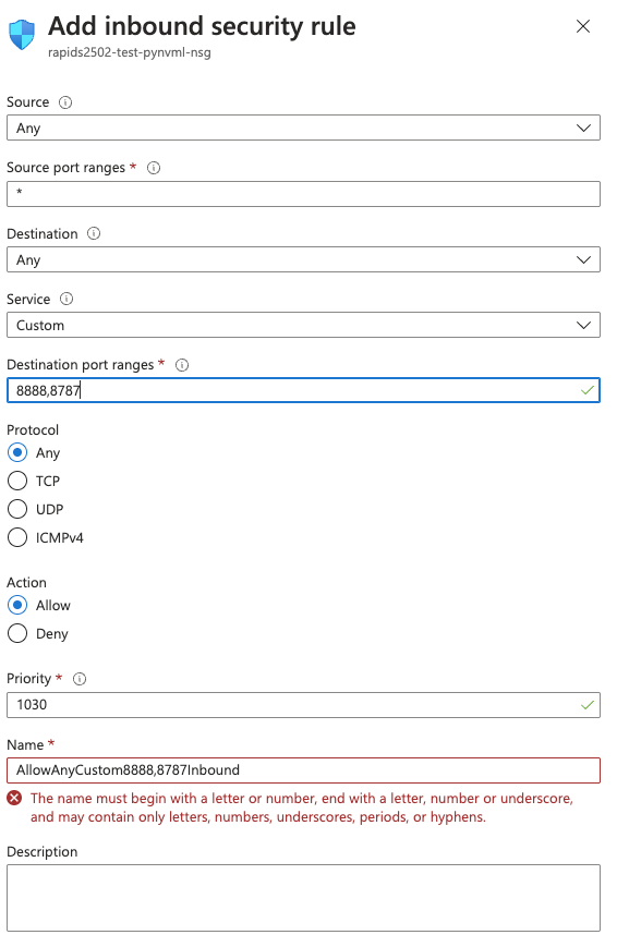
1. Keep rest unchanged. Select **Add**.
### via Azure CLI
| Name | Description | Example |
|------------------|---------------------|----------------------------|
| `AZ_NSGNAME` | NSG name for the VM | `${AZ_VMNAME}NSG` |
| `AZ_NSGRULENAME` | Name for NSG rule | `Allow-Dask-Jupyter-ports` |
```bash
$ az network nsg rule create \
-g ${AZ_RESOURCEGROUP} \
--nsg-name ${AZ_NSGNAME} \
-n ${AZ_NSGRULENAME} \
--priority 1050 \
--destination-port-ranges 8888 8787
```
## Install RAPIDS
Next, we can SSH into our VM to install RAPIDS. SSH instructions can be found by selecting **Connect** in the left panel.
There are a selection of methods you can use to install RAPIDS which you can see via the [RAPIDS release selector](https://docs.rapids.ai/install#selector).
For this example we are going to run the RAPIDS Docker container so we need to know the name of the most recent container.
On the release selector choose **Docker** in the **Method** column.
Then copy the commands shown:
```bash
docker pull rapidsai/notebooks:25.12a-cuda12-py3.13
docker run --gpus all --rm -it \
--shm-size=1g --ulimit memlock=-1 \
-p 8888:8888 -p 8787:8787 -p 8786:8786 \
rapidsai/notebooks:25.12a-cuda12-py3.13
```
#### NOTE
If you see a “docker socket permission denied” error while running these commands try closing and reconnecting your
SSH window. This happens because your user was added to the `docker` group only after you signed in.
## Test RAPIDS
To access Jupyter, navigate to `:8888` in the browser.
In a Python notebook, check that you can import and use RAPIDS libraries like `cudf`.
```ipython
In [1]: import cudf
In [2]: df = cudf.datasets.timeseries()
In [3]: df.head()
Out[3]:
id name x y
timestamp
2000-01-01 00:00:00 1020 Kevin 0.091536 0.664482
2000-01-01 00:00:01 974 Frank 0.683788 -0.467281
2000-01-01 00:00:02 1000 Charlie 0.419740 -0.796866
2000-01-01 00:00:03 1019 Edith 0.488411 0.731661
2000-01-01 00:00:04 998 Quinn 0.651381 -0.525398
```
Open `cudf/10min.ipynb` and execute the cells to explore more of how `cudf` works.
When running a Dask cluster you can also visit `:8787` to monitor the Dask cluster status.
### Useful Links
- [Using NGC with Azure](https://docs.nvidia.com/ngc/ngc-deploy-public-cloud/ngc-azure/index.html)
#### Related Examples
Measuring Performance with the One Billion Row Challenge
tools/dask-cuda
data-format/csv
library/cudf
library/cupy
library/dask
library/pandas
cloud/aws/ec2
cloud/aws/sagemaker
cloud/azure/azure-vm
cloud/azure/ml
cloud/gcp/compute-engine
cloud/gcp/vertex-ai
HPO with dask-ml and cuml
dataset/airline
library/numpy
library/pandas
library/xgboost
library/dask
library/dask-cuda
library/dask-ml
library/cuml
cloud/aws/ec2
cloud/azure/azure-vm
cloud/gcp/compute-engine
cloud/ibm/virtual-server
library/sklearn
data-storage/s3
workflow/hpo
# index.html.md
# Azure Machine Learning
RAPIDS can be deployed at scale using [Azure Machine Learning Service](https://learn.microsoft.com/en-us/azure/machine-learning/overview-what-is-azure-machine-learning) and can be scaled up to any size needed.
## Pre-requisites
Use existing or create new Azure Machine Learning workspace through the [Azure portal](https://learn.microsoft.com/en-us/azure/machine-learning/how-to-manage-workspace?tabs=azure-portal#create-a-workspace), [Azure ML Python SDK](https://learn.microsoft.com/en-us/azure/machine-learning/how-to-manage-workspace?tabs=python#create-a-workspace), [Azure CLI](https://learn.microsoft.com/en-us/azure/machine-learning/how-to-manage-workspace-cli?tabs=createnewresources) or [Azure Resource Manager templates](https://learn.microsoft.com/en-us/azure/machine-learning/how-to-create-workspace-template?tabs=azcli).
Follow these high-level steps to get started:
**1. Create.** Create your Azure Resource Group.
**2. Workspace.** Within the Resource Group, create an Azure Machine Learning service Workspace.
**3. Quota.** Check your subscription Usage + Quota to ensure you have enough quota within your region to launch your desired compute instance.
## Azure ML Compute instance
Although it is possible to install Azure Machine Learning on your local computer, it is recommended to utilize [Azure’s ML Compute instances](https://learn.microsoft.com/en-us/azure/machine-learning/concept-compute-instance), fully managed and secure development environments that can also serve as a [compute target](https://learn.microsoft.com/en-us/azure/machine-learning/concept-compute-target?view=azureml-api-2) for ML training.
The compute instance provides an integrated Jupyter notebook service, JupyterLab, Azure ML Python SDK, CLI, and other essential tools.
### Select your instance
Sign in to [Azure Machine Learning Studio](https://ml.azure.com/) and navigate to your workspace on the left-side menu.
Select **New** > **Compute instance** (Create compute instance) > choose an [Azure RAPIDS compatible GPU](https://docs.rapids.ai/deployment/stable/cloud/azure/) VM size (e.g., `Standard_NC12s_v3`)

### Provision RAPIDS setup script
Navigate to the **Applications** section.
Choose “Provision with a creation script” to install RAPIDS and dependencies.
Put the following in a local file called `rapids-azure-startup.sh`:
#### NOTE
The script below has `set -e` to avoid silent fails. In case of failure, remove this line
from the script, the VM will boot and inspect it by running each line of the script
to see where it fails.
```bash
#!/bin/bash
set -e
sudo -u azureuser -i <<'EOF'
source /anaconda/etc/profile.d/conda.sh
conda create -y -n rapids \
--override-channels \
-c rapidsai-nightly -c conda-forge -c nvidia \
-c microsoft \
rapids=25.12 python=3.13 'cuda-version>=12.0,<=12.9' \
'azure-identity>=1.19' \
ipykernel
conda activate rapids
pip install 'azure-ai-ml>=1.24'
python -m ipykernel install --user --name rapids
echo "kernel install completed"
EOF
```
Select `local file`, then `Browse`, and upload that script.

Refer to [Azure ML documentation](https://learn.microsoft.com/en-us/azure/machine-learning/how-to-customize-compute-instance) for more details on how to create the setup script.
Launch the instance.
### Select the RAPIDS environment
Once your Notebook Instance is `Running`, open “JupyterLab” and select the `rapids` kernel when working with a new notebook.
## Azure ML Compute cluster
In the next section we will launch Azure’s [ML Compute cluster](https://learn.microsoft.com/en-us/azure/machine-learning/how-to-create-attach-compute-cluster?tabs=python) to distribute your RAPIDS training jobs across a cluster of single or multi-GPU compute nodes.
The Compute cluster scales up automatically when a job is submitted, and executes in a containerized environment, packaging your model dependencies in a Docker container.
### Instantiate workspace
Use Azure’s client libraries to set up some resources.
```python
from azure.ai.ml import MLClient
from azure.identity import DefaultAzureCredential
# Get a handle to the workspace.
#
# Azure ML places the workspace config at the default working
# directory for notebooks by default.
#
# If it isn't found, open a shell and look in the
# directory indicated by 'echo ${JUPYTER_SERVER_ROOT}'.
ml_client = MLClient.from_config(
credential=DefaultAzureCredential(),
path="./config.json",
)
```
### Create AMLCompute
You will need to create a [compute target](https://learn.microsoft.com/en-us/azure/machine-learning/concept-compute-target?view=azureml-api-2#azure-machine-learning-compute-managed) using Azure ML managed compute ([AmlCompute](https://azuresdkdocs.blob.core.windows.net/$web/python/azure-ai-ml/0.1.0b4/azure.ai.ml.entities.html)) for remote training.
#### NOTE
Be sure to check instance availability and its limits within the region where you created your compute instance.
This [article](https://learn.microsoft.com/en-us/azure/machine-learning/how-to-manage-quotas?view=azureml-api-2#azure-machine-learning-compute) includes details on the default limits and how to request more quota.
[**size**]: The VM family of the nodes.
Specify from one of **NC_v2**, **NC_v3**, **ND** or **ND_v2** GPU virtual machines (e.g `Standard_NC12s_v3`)
[**max_instances**]: The max number of nodes to autoscale up to when you run a job
#### NOTE
You may choose to use low-priority VMs to run your workloads. These VMs don’t have guaranteed availability but allow you to take advantage of Azure’s unused capacity at a significant cost savings. The amount of available capacity can vary based on size, region, time of day, and more.
```python
from azure.ai.ml.entities import AmlCompute
gpu_compute = AmlCompute(
name="rapids-cluster",
type="amlcompute",
size="Standard_NC12s_v3", # this VM type needs to be available in your current region
max_instances=3,
idle_time_before_scale_down=300, # Seconds of idle time before scaling down
tier="low_priority", # optional
)
ml_client.begin_create_or_update(gpu_compute).result()
```
If you name your cluster `"rapids-cluster"` you can check [https://ml.azure.com/compute/rapids-cluster/details](https://ml.azure.com/compute/rapids-cluster/details)
to see the details about your cluster.
### Access Datastore URI
A [datastore URI](https://learn.microsoft.com/en-us/azure/machine-learning/how-to-access-data-interactive?tabs=adls&view=azureml-api-2#access-data-from-a-datastore-uri-like-a-filesystem-preview) is a reference to a blob storage location (path) on your Azure account. You can copy-and-paste the datastore URI from the AzureML Studio UI:
1. Select **Data** from the left-hand menu > **Datastores** > choose your datastore name > **Browse**
2. Find the file/folder containing your dataset and click the ellipsis (…) next to it.
3. From the menu, choose **Copy URI** and select **Datastore URI** format to copy into your notebook.

### Custom RAPIDS Environment
To run an AzureML experiment, you must specify an [environment](https://learn.microsoft.com/en-us/azure/machine-learning/concept-environments?view=azureml-api-2) that contains all the necessary software dependencies to run the training script on distributed nodes.
.
2. Click **Runtime** > **Run All**.
3. Wait a few minutes for the installation to complete without errors.
4. Add your code in the cells below the template.
## Section 2: User Customizable RAPIDS Install Instructions
### 1. Launch notebook
To get started in [Google Colab](https://colab.research.google.com/), click `File` at the top toolbar to Create new or Upload existing notebook
### 2. Set the Runtime
Click the `Runtime` dropdown and select `Change Runtime Type`

Choose GPU for Hardware Accelerator

### 3. Check GPU type
Check the output of `!nvidia-smi` to make sure you’ve been allocated a Rapids Compatible GPU ([see the RAPIDS install docs](https://docs.rapids.ai/install/#system-req)).

### 4. Install RAPIDS on Colab
You can install RAPIDS using pip. The script first checks GPU compatibility with RAPIDS, then installs the latest **stable** versions of some core RAPIDS libraries (e.g. cuDF, cuML, cuGraph, and xgboost) using `pip`.
```bash
# Colab warns and provides remediation steps if the GPUs is not compatible with RAPIDS.
!git clone https://github.com/rapidsai/rapidsai-csp-utils.git
!python rapidsai-csp-utils/colab/pip-install.py
```
### 5. Test RAPIDS
Run the following in a Python cell.
```python
import cudf
gdf = cudf.DataFrame({"a":[1,2,3], "b":[4,5,6]})
gdf
a b
0 1 4
1 2 5
2 3 6
```
### 6. Next steps
Try a more thorough example of using cuDF on Google Colab, “10 Minutes to RAPIDS cuDF’s pandas accelerator mode (cudf.pandas)” ([Google Colab link](https://nvda.ws/rapids-cudf)).
# index.html.md
# Continuous Integration
GitHub Actions
Run tests in GitHub Actions that depend on RAPIDS and NVIDIA GPUs.
single-node
# index.html.md
# Continuous Integration
GitHub Actions
Run tests in GitHub Actions that depend on RAPIDS and NVIDIA GPUs.
single-node
# index.html.md
# Virtual Server for VPC
## Create Instance
Create a new [Virtual Server (for VPC)](https://www.ibm.com/cloud/virtual-servers) with GPUs, the [NVIDIA Driver](https://www.nvidia.co.uk/Download/index.aspx) and the [NVIDIA Container Runtime](https://developer.nvidia.com/nvidia-container-runtime).
1. Open the [**Virtual Server Dashboard**](https://cloud.ibm.com/vpc-ext/compute/vs).
2. Select **Create**.
3. Give the server a **name** and select your **resource group**.
4. Under **Operating System** choose **Ubuntu Linux**.
5. Under **Profile** select **View all profiles** and select a profile with NVIDIA GPUs.
6. Under **SSH Keys** choose your SSH key.
7. Under network settings create a security group (or choose an existing) that allows SSH access on port `22` and also allow ports `8888,8786,8787` to access Jupyter and Dask.
8. Select **Create Virtual Server**.
## Create floating IP
To access the virtual server we need to attach a public IP address.
1. Open [**Floating IPs**](https://cloud.ibm.com/vpc-ext/network/floatingIPs)
2. Select **Reserve**.
3. Give the Floating IP a **name**.
4. Under **Resource to bind** select the virtual server you just created.
## Connect to the instance
Next we need to connect to the instance.
1. Open [**Floating IPs**](https://cloud.ibm.com/vpc-ext/network/floatingIPs)
2. Locate the IP you just created and note the address.
3. In your terminal run `ssh root@`
#### NOTE
For a short guide on launching your instance and accessing it, read the
[Getting Started with IBM Virtual Server Documentation](https://cloud.ibm.com/docs/virtual-servers?topic=virtual-servers-getting-started-tutorial).
## Install NVIDIA Drivers
Next we need to install the NVIDIA drivers and container runtime.
1. Ensure build essentials are installed `apt-get update && apt-get install build-essential -y`.
2. Install the [NVIDIA drivers](https://www.nvidia.com/Download/index.aspx?lang=en-us).
3. Install [Docker and the NVIDIA Docker runtime](https://docs.nvidia.com/datacenter/cloud-native/container-toolkit/install-guide.html).
### How do I check everything installed successfully?
You can check everything installed correctly by running `nvidia-smi` in a container.
```console
$ docker run --rm --gpus all nvidia/cuda:11.6.2-base-ubuntu20.04 nvidia-smi
+-----------------------------------------------------------------------------+
| NVIDIA-SMI 510.108.03 Driver Version: 510.108.03 CUDA Version: 11.6 |
|-------------------------------+----------------------+----------------------+
| GPU Name Persistence-M| Bus-Id Disp.A | Volatile Uncorr. ECC |
| Fan Temp Perf Pwr:Usage/Cap| Memory-Usage | GPU-Util Compute M. |
| | | MIG M. |
|===============================+======================+======================|
| 0 Tesla V100-PCIE... Off | 00000000:04:01.0 Off | 0 |
| N/A 33C P0 36W / 250W | 0MiB / 16384MiB | 0% Default |
| | | N/A |
+-------------------------------+----------------------+----------------------+
+-----------------------------------------------------------------------------+
| Processes: |
| GPU GI CI PID Type Process name GPU Memory |
| ID ID Usage |
|=============================================================================|
| No running processes found |
+-----------------------------------------------------------------------------+
```
## Install RAPIDS
There are a selection of methods you can use to install RAPIDS which you can see via the [RAPIDS release selector](https://docs.rapids.ai/install#selector).
For this example we are going to run the RAPIDS Docker container so we need to know the name of the most recent container.
On the release selector choose **Docker** in the **Method** column.
Then copy the commands shown:
```bash
docker pull rapidsai/notebooks:25.12a-cuda12-py3.13
docker run --gpus all --rm -it \
--shm-size=1g --ulimit memlock=-1 \
-p 8888:8888 -p 8787:8787 -p 8786:8786 \
rapidsai/notebooks:25.12a-cuda12-py3.13
```
#### NOTE
If you see a “docker socket permission denied” error while running these commands try closing and reconnecting your
SSH window. This happens because your user was added to the `docker` group only after you signed in.
## Test RAPIDS
To access Jupyter, navigate to `:8888` in the browser.
In a Python notebook, check that you can import and use RAPIDS libraries like `cudf`.
```ipython
In [1]: import cudf
In [2]: df = cudf.datasets.timeseries()
In [3]: df.head()
Out[3]:
id name x y
timestamp
2000-01-01 00:00:00 1020 Kevin 0.091536 0.664482
2000-01-01 00:00:01 974 Frank 0.683788 -0.467281
2000-01-01 00:00:02 1000 Charlie 0.419740 -0.796866
2000-01-01 00:00:03 1019 Edith 0.488411 0.731661
2000-01-01 00:00:04 998 Quinn 0.651381 -0.525398
```
Open `cudf/10min.ipynb` and execute the cells to explore more of how `cudf` works.
When running a Dask cluster you can also visit `:8787` to monitor the Dask cluster status.
### Related Examples
HPO with dask-ml and cuml
dataset/airline
library/numpy
library/pandas
library/xgboost
library/dask
library/dask-cuda
library/dask-ml
library/cuml
cloud/aws/ec2
cloud/azure/azure-vm
cloud/gcp/compute-engine
cloud/ibm/virtual-server
library/sklearn
data-storage/s3
workflow/hpo
# index.html.md
# Azure Virtual Machine
## Create Virtual Machine
Create a new [Azure Virtual Machine](https://azure.microsoft.com/en-gb/products/virtual-machines/) with GPUs, the [NVIDIA Driver](https://www.nvidia.co.uk/Download/index.aspx) and the [NVIDIA Container Runtime](https://developer.nvidia.com/nvidia-container-runtime).
NVIDIA maintains a [Virtual Machine Image (VMI) that pre-installs NVIDIA drivers and container runtimes](https://azuremarketplace.microsoft.com/en-us/marketplace/apps/nvidia.ngc_azure_17_11?tab=Overview), we recommend using this image as the starting point.
### via Azure Portal
1. Select a resource group or create one if needed.
2. Select the latest **NVIDIA GPU-Optimized VMI** version from the drop down list, then select **Get It Now** (if there are multiple `Gen` versions, select the latest).
3. If already logged in on Azure, select continue clicking **Create**.
4. In **Create a virtual machine** interface, fill in required information for the vm.
- Select a GPU enabled VM size (see [recommended VM types](https://docs.rapids.ai/deployment/stable/cloud/azure/)).
- In “Configure security features” select Standard.
- Make sure you create ssh keys and download them.
### Note that not all regions support availability zones with GPU VMs.
When the GPU VM size is not selectable
with notice: **The size is not available in zone x. No zones are supported.** It means the GPU VM does not
support availability zone. Try other availability options.

Click **Review+Create** to start the virtual machine.
### via Azure CLI
Prepare the following environment variables.
| Name | Description | Example |
|--------------------|----------------------|----------------------------------------------------------------|
| `AZ_VMNAME` | Name for VM | `RapidsAI-V100` |
| `AZ_RESOURCEGROUP` | Resource group of VM | `rapidsai-deployment` |
| `AZ_LOCATION` | Region of VM | `westus2` |
| `AZ_IMAGE` | URN of image | `nvidia:ngc_azure_17_11:ngc-base-version-22_06_0-gen2:22.06.0` |
| `AZ_SIZE` | VM Size | `Standard_NC6s_v3` |
| `AZ_USERNAME` | User name of VM | `rapidsai` |
| `AZ_SSH_KEY` | public ssh key | `~/.ssh/id_rsa.pub` |
```bash
$ az vm create \
--name ${AZ_VMNAME} \
--resource-group ${AZ_RESOURCEGROUP} \
--image ${AZ_IMAGE} \
--location ${AZ_LOCATION} \
--size ${AZ_SIZE} \
--admin-username ${AZ_USERNAME} \
--ssh-key-value ${AZ_SSH_KEY}
```
#### NOTE
Use `az vm image list --publisher Nvidia --all --output table` to inspect URNs of official
NVIDIA images on Azure.
#### NOTE
See [this link](https://learn.microsoft.com/en-us/azure/virtual-machines/linux/mac-create-ssh-keys)
for supported ssh keys on Azure.
## Create Network Security Group
Next we need to allow network traffic to the VM so we can access Jupyter and Dask.
### via Azure Portal
1. After creating VM, select **Go to resource** to access VM.
2. Select **Networking** -> **Networking Settings** in the left panel.
3. Select **+Create port rule** -> **Add inbound port rule**.
4. Set **Destination port ranges** to `8888,8787`.
5. Modify the “Name” to avoid the `,` or any other symbols.
### See example of port setting.

1. Keep rest unchanged. Select **Add**.
### via Azure CLI
| Name | Description | Example |
|------------------|---------------------|----------------------------|
| `AZ_NSGNAME` | NSG name for the VM | `${AZ_VMNAME}NSG` |
| `AZ_NSGRULENAME` | Name for NSG rule | `Allow-Dask-Jupyter-ports` |
```bash
$ az network nsg rule create \
-g ${AZ_RESOURCEGROUP} \
--nsg-name ${AZ_NSGNAME} \
-n ${AZ_NSGRULENAME} \
--priority 1050 \
--destination-port-ranges 8888 8787
```
## Install RAPIDS
Next, we can SSH into our VM to install RAPIDS. SSH instructions can be found by selecting **Connect** in the left panel.
There are a selection of methods you can use to install RAPIDS which you can see via the [RAPIDS release selector](https://docs.rapids.ai/install#selector).
For this example we are going to run the RAPIDS Docker container so we need to know the name of the most recent container.
On the release selector choose **Docker** in the **Method** column.
Then copy the commands shown:
```bash
docker pull rapidsai/notebooks:25.12a-cuda12-py3.13
docker run --gpus all --rm -it \
--shm-size=1g --ulimit memlock=-1 \
-p 8888:8888 -p 8787:8787 -p 8786:8786 \
rapidsai/notebooks:25.12a-cuda12-py3.13
```
#### NOTE
If you see a “docker socket permission denied” error while running these commands try closing and reconnecting your
SSH window. This happens because your user was added to the `docker` group only after you signed in.
## Test RAPIDS
To access Jupyter, navigate to `:8888` in the browser.
In a Python notebook, check that you can import and use RAPIDS libraries like `cudf`.
```ipython
In [1]: import cudf
In [2]: df = cudf.datasets.timeseries()
In [3]: df.head()
Out[3]:
id name x y
timestamp
2000-01-01 00:00:00 1020 Kevin 0.091536 0.664482
2000-01-01 00:00:01 974 Frank 0.683788 -0.467281
2000-01-01 00:00:02 1000 Charlie 0.419740 -0.796866
2000-01-01 00:00:03 1019 Edith 0.488411 0.731661
2000-01-01 00:00:04 998 Quinn 0.651381 -0.525398
```
Open `cudf/10min.ipynb` and execute the cells to explore more of how `cudf` works.
When running a Dask cluster you can also visit `:8787` to monitor the Dask cluster status.
### Useful Links
- [Using NGC with Azure](https://docs.nvidia.com/ngc/ngc-deploy-public-cloud/ngc-azure/index.html)
#### Related Examples
Measuring Performance with the One Billion Row Challenge
tools/dask-cuda
data-format/csv
library/cudf
library/cupy
library/dask
library/pandas
cloud/aws/ec2
cloud/aws/sagemaker
cloud/azure/azure-vm
cloud/azure/ml
cloud/gcp/compute-engine
cloud/gcp/vertex-ai
HPO with dask-ml and cuml
dataset/airline
library/numpy
library/pandas
library/xgboost
library/dask
library/dask-cuda
library/dask-ml
library/cuml
cloud/aws/ec2
cloud/azure/azure-vm
cloud/gcp/compute-engine
cloud/ibm/virtual-server
library/sklearn
data-storage/s3
workflow/hpo
# index.html.md
# Azure Machine Learning
RAPIDS can be deployed at scale using [Azure Machine Learning Service](https://learn.microsoft.com/en-us/azure/machine-learning/overview-what-is-azure-machine-learning) and can be scaled up to any size needed.
## Pre-requisites
Use existing or create new Azure Machine Learning workspace through the [Azure portal](https://learn.microsoft.com/en-us/azure/machine-learning/how-to-manage-workspace?tabs=azure-portal#create-a-workspace), [Azure ML Python SDK](https://learn.microsoft.com/en-us/azure/machine-learning/how-to-manage-workspace?tabs=python#create-a-workspace), [Azure CLI](https://learn.microsoft.com/en-us/azure/machine-learning/how-to-manage-workspace-cli?tabs=createnewresources) or [Azure Resource Manager templates](https://learn.microsoft.com/en-us/azure/machine-learning/how-to-create-workspace-template?tabs=azcli).
Follow these high-level steps to get started:
**1. Create.** Create your Azure Resource Group.
**2. Workspace.** Within the Resource Group, create an Azure Machine Learning service Workspace.
**3. Quota.** Check your subscription Usage + Quota to ensure you have enough quota within your region to launch your desired compute instance.
## Azure ML Compute instance
Although it is possible to install Azure Machine Learning on your local computer, it is recommended to utilize [Azure’s ML Compute instances](https://learn.microsoft.com/en-us/azure/machine-learning/concept-compute-instance), fully managed and secure development environments that can also serve as a [compute target](https://learn.microsoft.com/en-us/azure/machine-learning/concept-compute-target?view=azureml-api-2) for ML training.
The compute instance provides an integrated Jupyter notebook service, JupyterLab, Azure ML Python SDK, CLI, and other essential tools.
### Select your instance
Sign in to [Azure Machine Learning Studio](https://ml.azure.com/) and navigate to your workspace on the left-side menu.
Select **New** > **Compute instance** (Create compute instance) > choose an [Azure RAPIDS compatible GPU](https://docs.rapids.ai/deployment/stable/cloud/azure/) VM size (e.g., `Standard_NC12s_v3`)

### Provision RAPIDS setup script
Navigate to the **Applications** section.
Choose “Provision with a creation script” to install RAPIDS and dependencies.
Put the following in a local file called `rapids-azure-startup.sh`:
#### NOTE
The script below has `set -e` to avoid silent fails. In case of failure, remove this line
from the script, the VM will boot and inspect it by running each line of the script
to see where it fails.
```bash
#!/bin/bash
set -e
sudo -u azureuser -i <<'EOF'
source /anaconda/etc/profile.d/conda.sh
conda create -y -n rapids \
--override-channels \
-c rapidsai-nightly -c conda-forge -c nvidia \
-c microsoft \
rapids=25.12 python=3.13 'cuda-version>=12.0,<=12.9' \
'azure-identity>=1.19' \
ipykernel
conda activate rapids
pip install 'azure-ai-ml>=1.24'
python -m ipykernel install --user --name rapids
echo "kernel install completed"
EOF
```
Select `local file`, then `Browse`, and upload that script.

Refer to [Azure ML documentation](https://learn.microsoft.com/en-us/azure/machine-learning/how-to-customize-compute-instance) for more details on how to create the setup script.
Launch the instance.
### Select the RAPIDS environment
Once your Notebook Instance is `Running`, open “JupyterLab” and select the `rapids` kernel when working with a new notebook.
## Azure ML Compute cluster
In the next section we will launch Azure’s [ML Compute cluster](https://learn.microsoft.com/en-us/azure/machine-learning/how-to-create-attach-compute-cluster?tabs=python) to distribute your RAPIDS training jobs across a cluster of single or multi-GPU compute nodes.
The Compute cluster scales up automatically when a job is submitted, and executes in a containerized environment, packaging your model dependencies in a Docker container.
### Instantiate workspace
Use Azure’s client libraries to set up some resources.
```python
from azure.ai.ml import MLClient
from azure.identity import DefaultAzureCredential
# Get a handle to the workspace.
#
# Azure ML places the workspace config at the default working
# directory for notebooks by default.
#
# If it isn't found, open a shell and look in the
# directory indicated by 'echo ${JUPYTER_SERVER_ROOT}'.
ml_client = MLClient.from_config(
credential=DefaultAzureCredential(),
path="./config.json",
)
```
### Create AMLCompute
You will need to create a [compute target](https://learn.microsoft.com/en-us/azure/machine-learning/concept-compute-target?view=azureml-api-2#azure-machine-learning-compute-managed) using Azure ML managed compute ([AmlCompute](https://azuresdkdocs.blob.core.windows.net/$web/python/azure-ai-ml/0.1.0b4/azure.ai.ml.entities.html)) for remote training.
#### NOTE
Be sure to check instance availability and its limits within the region where you created your compute instance.
This [article](https://learn.microsoft.com/en-us/azure/machine-learning/how-to-manage-quotas?view=azureml-api-2#azure-machine-learning-compute) includes details on the default limits and how to request more quota.
[**size**]: The VM family of the nodes.
Specify from one of **NC_v2**, **NC_v3**, **ND** or **ND_v2** GPU virtual machines (e.g `Standard_NC12s_v3`)
[**max_instances**]: The max number of nodes to autoscale up to when you run a job
#### NOTE
You may choose to use low-priority VMs to run your workloads. These VMs don’t have guaranteed availability but allow you to take advantage of Azure’s unused capacity at a significant cost savings. The amount of available capacity can vary based on size, region, time of day, and more.
```python
from azure.ai.ml.entities import AmlCompute
gpu_compute = AmlCompute(
name="rapids-cluster",
type="amlcompute",
size="Standard_NC12s_v3", # this VM type needs to be available in your current region
max_instances=3,
idle_time_before_scale_down=300, # Seconds of idle time before scaling down
tier="low_priority", # optional
)
ml_client.begin_create_or_update(gpu_compute).result()
```
If you name your cluster `"rapids-cluster"` you can check [https://ml.azure.com/compute/rapids-cluster/details](https://ml.azure.com/compute/rapids-cluster/details)
to see the details about your cluster.
### Access Datastore URI
A [datastore URI](https://learn.microsoft.com/en-us/azure/machine-learning/how-to-access-data-interactive?tabs=adls&view=azureml-api-2#access-data-from-a-datastore-uri-like-a-filesystem-preview) is a reference to a blob storage location (path) on your Azure account. You can copy-and-paste the datastore URI from the AzureML Studio UI:
1. Select **Data** from the left-hand menu > **Datastores** > choose your datastore name > **Browse**
2. Find the file/folder containing your dataset and click the ellipsis (…) next to it.
3. From the menu, choose **Copy URI** and select **Datastore URI** format to copy into your notebook.

### Custom RAPIDS Environment
To run an AzureML experiment, you must specify an [environment](https://learn.microsoft.com/en-us/azure/machine-learning/concept-environments?view=azureml-api-2) that contains all the necessary software dependencies to run the training script on distributed nodes.
You can define an environment from a [pre-built](https://learn.microsoft.com/en-us/azure/machine-learning/how-to-manage-environments-v2?tabs=python&view=azureml-api-2#create-an-environment-from-a-docker-image) docker image or create-your-own from a [Dockerfile](https://learn.microsoft.com/en-us/azure/machine-learning/how-to-manage-environments-v2?tabs=python&view=azureml-api-2#create-an-environment-from-a-docker-build-context) or [conda](https://learn.microsoft.com/en-us/azure/machine-learning/how-to-manage-environments-v2?tabs=python&view=azureml-api-2#create-an-environment-from-a-conda-specification) specification file.
In a notebook cell, run the following to copy the example code from this documentation into a new folder,
and to create a Dockerfile to build and image that starts from a RAPIDS image and install additional packages needed for the
workflow.
```ipython
%%bash
mkdir -p ./training-code
repo_url='https://raw.githubusercontent.com/rapidsai/deployment/refs/heads/main/source/examples'
# download training scripts
wget -O ./training-code/train_rapids.py "${repo_url}/rapids-azureml-hpo/train_rapids.py"
wget -O ./training-code/rapids_csp_azure.py "${repo_url}/rapids-azureml-hpo/rapids_csp_azure.py"
touch ./training-code/__init__.py
# create a Dockerfile defining the image the code will run in
cat > ./training-code/Dockerfile <=2024.4.4' \
&& pip install azureml-mlflow
EOF
```
Now create the Environment, making sure to label and provide a description:
```python
from azure.ai.ml.entities import Environment, BuildContext
# NOTE: 'path' should be a filepath pointing to a directory containing a file named 'Dockerfile'
env_docker_image = Environment(
build=BuildContext(path="./training-code/"),
name="rapids-mlflow", # label
description="RAPIDS environment with azureml-mlflow",
)
ml_client.environments.create_or_update(env_docker_image)
```
### Submit RAPIDS Training jobs
Now that we have our environment and custom logic, we can configure and run the `command` [class](https://learn.microsoft.com/en-us/python/api/azure-ai-ml/azure.ai.ml?view=azure-python#azure-ai-ml-command) to submit training jobs.
`inputs` is a dictionary of command-line arguments to pass to the training script.
```python
from azure.ai.ml import command, Input
# replace this with your own dataset
datastore_name = "workspaceartifactstore"
dataset = "airline_20000000.parquet"
data_uri = f"azureml://subscriptions/{ml_client.subscription_id}/resourcegroups/{ml_client.resource_group_name}/workspaces/{ml_client.workspace_name}/datastores/{datastore_name}/paths/{dataset}"
command_job = command(
environment=f"{env_docker_image.name}:{env_docker_image.version}",
experiment_name="test_rapids_mlflow",
code="./training-code",
command="python train_rapids.py \
--data_dir ${{inputs.data_dir}} \
--n_bins ${{inputs.n_bins}} \
--cv_folds ${{inputs.cv_folds}} \
--n_estimators ${{inputs.n_estimators}} \
--max_depth ${{inputs.max_depth}} \
--max_features ${{inputs.max_features}}",
inputs={
"data_dir": Input(type="uri_file", path=data_uri),
"n_bins": 32,
"cv_folds": 5,
"n_estimators": 50,
"max_depth": 10,
"max_features": 1.0,
},
compute=gpu_compute.name,
)
# submit training job
returned_job = ml_client.jobs.create_or_update(command_job)
returned_job # displays status and details page of the experiment
```
After creating the job, click on the details page provided in the output of `returned_job`, or go
to [the “Experiments” page](https://ml.azure.com/experiments) to view logs, metrics, and outputs.
#### NOTE
For reference this job took ~7 min while using `size="Standard_NC6s_v3"` in the `gpu_compute` creation

Next, we can perform a sweep over a set of hyperparameters.
```python
from azure.ai.ml.sweep import Choice, Uniform
# define hyperparameter space to sweep over
command_job_for_sweep = command_job(
n_estimators=Choice(values=range(50, 500)),
max_depth=Choice(values=range(5, 19)),
max_features=Uniform(min_value=0.2, max_value=1.0),
)
# apply hyperparameter sweep_job
sweep_job = command_job_for_sweep.sweep(
compute=gpu_compute.name,
sampling_algorithm="random",
primary_metric="Accuracy",
goal="Maximize",
)
# setting a very small limit of trials for demo purposes
sweep_job.set_limits(
max_total_trials=3, max_concurrent_trials=3, timeout=18000, trial_timeout=3600
)
# submit job
returned_sweep_job = ml_client.create_or_update(sweep_job)
returned_sweep_job
```
Once the job is created, click on the details page provided in the output of `returned_sweep_job`, or go
to [the “Experiments” page](https://ml.azure.com/experiments) to view logs, metrics, and outputs. The three trials
set in the `sweep_job.set_limits(...)` take between 20-40 min to complete when using `size="Standard_NC6s_v3"`.
### Clean Up
When you’re done, remove the compute resources.
```python
ml_client.compute.begin_delete(gpu_compute.name).wait()
```
Then check [https://ml.azure.com/compute/list/instances](https://ml.azure.com/compute/list/instances) and make sure your compute instance
is also stopped, and deleted if desired.
# index.html.md
# Continuous Integration
GitHub Actions
Run tests in GitHub Actions that depend on RAPIDS and NVIDIA GPUs.
single-node
# index.html.md
# Azure VM Cluster (via Dask)
## Create a Cluster using Dask Cloud Provider
The easiest way to setup a multi-node, multi-GPU cluster on Azure is to use [Dask Cloud Provider](https://cloudprovider.dask.org/en/latest/azure.html).
### 1. Install Dask Cloud Provider
Dask Cloud Provider can be installed via `conda` or `pip`. The Azure-specific capabilities will need to be installed via the `[azure]` pip extra.
```shell
$ pip install dask-cloudprovider[azure]
```
### 2. Configure your Azure Resources
Set up your [Azure Resource Group](https://cloudprovider.dask.org/en/latest/azure.html#resource-groups), [Virtual Network](https://cloudprovider.dask.org/en/latest/azure.html#virtual-networks), and [Security Group](https://cloudprovider.dask.org/en/latest/azure.html#security-groups) according to [Dask Cloud Provider instructions](https://cloudprovider.dask.org/en/latest/azure.html#authentication).
### 3. Create a Cluster
In Python terminal, a cluster can be created using the `dask_cloudprovider` package. The below example creates a cluster with 2 workers in `westus2` with `Standard_NC12s_v3` VMs. The VMs should have at least 100GB of disk space in order to accommodate the RAPIDS container image and related dependencies.
```python
from dask_cloudprovider.azure import AzureVMCluster
resource_group = ""
vnet = ""
security_group = ""
subscription_id = ""
cluster = AzureVMCluster(
resource_group=resource_group,
vnet=vnet,
security_group=security_group,
subscription_id=subscription_id,
location="westus2",
vm_size="Standard_NC12s_v3",
public_ingress=True,
disk_size=100,
n_workers=2,
worker_class="dask_cuda.CUDAWorker",
docker_image="rapidsai/base:25.12a-cuda12-py3.13",
docker_args="-p 8787:8787 -p 8786:8786",
)
```
### 4. Test RAPIDS
To test RAPIDS, create a distributed client for the cluster and query for the GPU model.
```python
from dask.distributed import Client
client = Client(cluster)
def get_gpu_model():
import pynvml
pynvml.nvmlInit()
return pynvml.nvmlDeviceGetName(pynvml.nvmlDeviceGetHandleByIndex(0))
client.submit(get_gpu_model).result()
```
```shell
Out[5]: b'Tesla V100-PCIE-16GB'
```
### 5. Cleanup
Once done with the cluster, ensure the `cluster` and `client` are closed:
```python
client.close()
cluster.close()
```
#### Related Examples
Multi-Node Multi-GPU XGBoost Example on Azure using dask-cloudprovider
cloud/azure/azure-vm-multi
tools/dask-cloudprovider
library/cudf
library/cuml
library/xgboost
library/dask
library/fil
data-storage/azure-data-lake
dataset/nyc-taxi
workflow/xgboost
# index.html.md
# Azure Kubernetes Service
RAPIDS can be deployed on Azure via the [Azure Kubernetes Service](https://azure.microsoft.com/en-us/products/kubernetes-service/) (AKS).
To run RAPIDS you’ll need a Kubernetes cluster with GPUs available.
## Prerequisites
First you’ll need to have the [`az` CLI tool](https://learn.microsoft.com/en-us/cli/azure/install-azure-cli) installed along with [`kubectl`](https://kubernetes.io/docs/tasks/tools/), [`helm`](https://helm.sh/docs/intro/install/), etc for managing Kubernetes.
Ensure you are logged into the `az` CLI.
```bash
$ az login
```
## Create the Kubernetes cluster
Now we can launch a GPU enabled AKS cluster. First launch an AKS cluster.
```bash
$ az aks create -g -n rapids \
--enable-managed-identity \
--node-count 1 \
--enable-addons monitoring \
--enable-msi-auth-for-monitoring \
--generate-ssh-keys
```
Once the cluster has created we need to pull the credentials into our local config.
```console
$ az aks get-credentials -g --name rapids
Merged "rapids" as current context in ~/.kube/config
```
Next we need to add an additional node group with GPUs which you can [learn more about in the Azure docs](https://learn.microsoft.com/en-us/azure/aks/gpu-cluster).
#### NOTE
You will need the `GPUDedicatedVHDPreview` feature enabled so that NVIDIA drivers are installed automatically.
You can check if this is enabled with:
```console
$ az feature list -o table --query "[?contains(name, 'Microsoft.ContainerService/GPUDedicatedVHDPreview')].{Name:name,State:properties.state}"
Name State
------------------------------------------------- -------------
Microsoft.ContainerService/GPUDedicatedVHDPreview NotRegistered
```
### If you see NotRegistered follow these instructions
If it is not registered for you you’ll need to register it which can take a few minutes.
```console
$ az feature register --name GPUDedicatedVHDPreview --namespace Microsoft.ContainerService
Once the feature 'GPUDedicatedVHDPreview' is registered, invoking 'az provider register -n Microsoft.ContainerService' is required to get the change propagated
Name
-------------------------------------------------
Microsoft.ContainerService/GPUDedicatedVHDPreview
```
Keep checking until it does into a registered state.
```console
$ az feature list -o table --query "[?contains(name, 'Microsoft.ContainerService/GPUDedicatedVHDPreview')].{Name:name,State:properties.state}"
Name State
------------------------------------------------- -----------
Microsoft.ContainerService/GPUDedicatedVHDPreview Registered
```
When the status shows as registered, refresh the registration of the `Microsoft.ContainerService` resource provider by using the `az provider register` command:
```bash
$ az provider register --namespace Microsoft.ContainerService
```
Then install the aks-preview CLI extension, use the following Azure CLI commands:
```bash
$ az extension add --name aks-preview
```
```bash
$ az aks nodepool add \
--resource-group \
--cluster-name rapids \
--name gpunp \
--node-count 1 \
--node-vm-size Standard_NC48ads_A100_v4 \
--enable-cluster-autoscaler \
--min-count 1 \
--max-count 3
```
Here we have added a new pool made up of `Standard_NC48ads_A100_v4` instances which each have two A100 GPUs. We’ve also enabled autoscaling between one and three nodes on the pool.
Then we can install the NVIDIA drivers.
```bash
$ helm install --wait --generate-name --repo https://helm.ngc.nvidia.com/nvidia \
-n gpu-operator --create-namespace \
gpu-operator \
--set operator.runtimeClass=nvidia-container-runtime
```
Once our new pool has been created and configured, we can test the cluster.
Let’s create a sample Pod that uses some GPU compute to make sure that everything is working as expected.
```bash
cat << EOF | kubectl create -f -
apiVersion: v1
kind: Pod
metadata:
name: cuda-vectoradd
spec:
restartPolicy: OnFailure
containers:
- name: cuda-vectoradd
image: "nvidia/samples:vectoradd-cuda11.6.0-ubuntu18.04"
resources:
limits:
nvidia.com/gpu: 1
EOF
```
```console
$ kubectl logs pod/cuda-vectoradd
[Vector addition of 50000 elements]
Copy input data from the host memory to the CUDA device
CUDA kernel launch with 196 blocks of 256 threads
Copy output data from the CUDA device to the host memory
Test PASSED
Done
```
If you see `Test PASSED` in the output, you can be confident that your Kubernetes cluster has GPU compute set up correctly.
Next, clean up that Pod.
```console
$ kubectl delete pod cuda-vectoradd
pod "cuda-vectoradd" deleted
```
we should be able to test that we can schedule GPU pods.
## Install RAPIDS
Now that you have a GPU enables Kubernetes cluster on AKS you can install RAPIDS with [any of the supported methods](../../platforms/kubernetes.md).
## Clean up
You can also delete the AKS cluster to stop billing with the following command.
```console
$ az aks delete -g -n rapids
/ Running ..
```
# index.html.md
# Compute Engine Instance
## Create Virtual Machine
Create a new [Compute Engine Instance](https://cloud.google.com/compute/docs/instances) with GPUs, the [NVIDIA Driver](https://www.nvidia.co.uk/Download/index.aspx) and the [NVIDIA Container Runtime](https://developer.nvidia.com/nvidia-container-runtime).
NVIDIA maintains a [Virtual Machine Image (VMI) that pre-installs NVIDIA drivers and container runtimes](https://console.cloud.google.com/marketplace/product/nvidia-ngc-public/nvidia-gpu-optimized-vmi), we recommend using this image.
1. Open [**Compute Engine**](https://console.cloud.google.com/compute/instances).
2. Select **Create Instance**.
3. Select the **Create VM from..** option at the top.
4. Select **Marketplace**.
5. Search for “nvidia” and select **NVIDIA GPU-Optimized VMI**, then select **Launch**.
6. In the **New NVIDIA GPU-Optimized VMI deployment** interface, fill in the name and any required information for the vm (the defaults should be fine for most users).
7. **Read and accept** the Terms of Service
8. Select **Deploy** to start the virtual machine.
## Allow network access
To access Jupyter and Dask we will need to set up some firewall rules to open up some ports.
### Create the firewall rule
1. Open [**VPC Network**](https://console.cloud.google.com/networking/networks/list).
2. Select **Firewall** and **Create firewall rule**
3. Give the rule a name like `rapids` and ensure the network matches the one you selected for the VM.
4. Add a tag like `rapids` which we will use to assign the rule to our VM.
5. Set your source IP range. We recommend you restrict this to your own IP address or your corporate network rather than `0.0.0.0/0` which will allow anyone to access your VM.
6. Under **Protocols and ports** allow TCP connections on ports `22,8786,8787,8888`.
### Assign it to the VM
1. Open [**Compute Engine**](https://console.cloud.google.com/compute/instances).
2. Select your VM and press **Edit**.
3. Scroll down to **Networking** and add the `rapids` network tag you gave your firewall rule.
4. Select **Save**.
## Connect to the VM
Next we need to connect to the VM.
1. Open [**Compute Engine**](https://console.cloud.google.com/compute/instances).
2. Locate your VM and press the **SSH** button which will open a new browser tab with a terminal.
3. **Read and accept** the NVIDIA installer prompts.
## Install RAPIDS
There are a selection of methods you can use to install RAPIDS which you can see via the [RAPIDS release selector](https://docs.rapids.ai/install#selector).
For this example we are going to run the RAPIDS Docker container so we need to know the name of the most recent container.
On the release selector choose **Docker** in the **Method** column.
Then copy the commands shown:
```bash
docker pull rapidsai/notebooks:25.12a-cuda12-py3.13
docker run --gpus all --rm -it \
--shm-size=1g --ulimit memlock=-1 \
-p 8888:8888 -p 8787:8787 -p 8786:8786 \
rapidsai/notebooks:25.12a-cuda12-py3.13
```
#### NOTE
If you see a “docker socket permission denied” error while running these commands try closing and reconnecting your
SSH window. This happens because your user was added to the `docker` group only after you signed in.
## Test RAPIDS
To access Jupyter, navigate to `:8888` in the browser.
In a Python notebook, check that you can import and use RAPIDS libraries like `cudf`.
```ipython
In [1]: import cudf
In [2]: df = cudf.datasets.timeseries()
In [3]: df.head()
Out[3]:
id name x y
timestamp
2000-01-01 00:00:00 1020 Kevin 0.091536 0.664482
2000-01-01 00:00:01 974 Frank 0.683788 -0.467281
2000-01-01 00:00:02 1000 Charlie 0.419740 -0.796866
2000-01-01 00:00:03 1019 Edith 0.488411 0.731661
2000-01-01 00:00:04 998 Quinn 0.651381 -0.525398
```
Open `cudf/10min.ipynb` and execute the cells to explore more of how `cudf` works.
When running a Dask cluster you can also visit `:8787` to monitor the Dask cluster status.
## Clean up
Once you are finished head back to the [Deployments](https://console.cloud.google.com/dm/deployments) page and delete the marketplace deployment you created.
### Related Examples
Measuring Performance with the One Billion Row Challenge
tools/dask-cuda
data-format/csv
library/cudf
library/cupy
library/dask
library/pandas
cloud/aws/ec2
cloud/aws/sagemaker
cloud/azure/azure-vm
cloud/azure/ml
cloud/gcp/compute-engine
cloud/gcp/vertex-ai
HPO with dask-ml and cuml
dataset/airline
library/numpy
library/pandas
library/xgboost
library/dask
library/dask-cuda
library/dask-ml
library/cuml
cloud/aws/ec2
cloud/azure/azure-vm
cloud/gcp/compute-engine
cloud/ibm/virtual-server
library/sklearn
data-storage/s3
workflow/hpo
# index.html.md
# Vertex AI
RAPIDS can be deployed on [Vertex AI Workbench](https://cloud.google.com/vertex-ai-workbench).
## Create a new Notebook Instance
1. From the Google Cloud UI, navigate to [**Vertex AI**](https://console.cloud.google.com/vertex-ai/workbench/user-managed) -> Notebook -> **Workbench**
2. Select **Instances** and select **+ CREATE NEW**.
3. In the **Details** section give the instance a name.
4. Check the “Attach 1 NVIDIA T4 GPU” option.
5. After customizing any other aspects of the machine you wish, click **CREATE**.
## Install RAPIDS
Once the instance has started select **OPEN JUPYTER LAB** and at the top of a notebook install the RAPIDS libraries you wish to use.
#### WARNING
Installing RAPIDS via `pip` in the default environment is [not currently possible](https://github.com/rapidsai/deployment/issues/517), for now you must create a new `conda` environment.
Vertex AI currently ships with CUDA Toolkit 11 system packages as of the [Jan 2025 Vertex AI release](https://cloud.google.com/vertex-ai/docs/release-notes#January_31_2025).
The default Python environment also contains the `cupy-cuda12x` package. This means it’s not possible to install RAPIDS package like `cudf` via `pip` as `cudf-cu12` will conflict with the CUDA Toolkit version but `cudf-cu11` will conflict with the `cupy` version.
You can find out your current system CUDA Toolkit version by running `ls -ld /usr/local/cuda*`.
You can create a new RAPIDS conda environment and register it with `ipykernel` for use in Jupyter Lab. Open a new terminal in Jupyter and run the following commands.
```bash
# Create a new environment
$ conda create -y -n rapids \
-c rapidsai-nightly -c conda-forge -c nvidia \
rapids=25.12 python=3.13 'cuda-version>=12.0,<=12.9' \
ipykernel
```
```bash
# Activate the environment
$ conda activate rapids
```
```bash
# Register the environment with Jupyter
$ python -m ipykernel install --prefix "${DL_ANACONDA_HOME}/envs/rapids" --name rapids --display-name rapids
```
Then refresh the Jupyter Lab page and open the launcher. You will see a new “rapids” kernel available.

## Test RAPIDS
You should now be able to open a notebook and use RAPIDS.
For example we could import and use RAPIDS libraries like `cudf`.
```ipython
In [1]: import cudf
In [2]: df = cudf.datasets.timeseries()
In [3]: df.head()
Out[3]:
id name x y
timestamp
2000-01-01 00:00:00 1020 Kevin 0.091536 0.664482
2000-01-01 00:00:01 974 Frank 0.683788 -0.467281
2000-01-01 00:00:02 1000 Charlie 0.419740 -0.796866
2000-01-01 00:00:03 1019 Edith 0.488411 0.731661
2000-01-01 00:00:04 998 Quinn 0.651381 -0.525398
```
### Related Examples
Measuring Performance with the One Billion Row Challenge
tools/dask-cuda
data-format/csv
library/cudf
library/cupy
library/dask
library/pandas
cloud/aws/ec2
cloud/aws/sagemaker
cloud/azure/azure-vm
cloud/azure/ml
cloud/gcp/compute-engine
cloud/gcp/vertex-ai
# index.html.md
# Continuous Integration
GitHub Actions
Run tests in GitHub Actions that depend on RAPIDS and NVIDIA GPUs.
single-node
# index.html.md
# Google Kubernetes Engine
RAPIDS can be deployed on Google Cloud via the [Google Kubernetes Engine](https://cloud.google.com/kubernetes-engine) (GKE).
To run RAPIDS you’ll need a Kubernetes cluster with GPUs available.
## Prerequisites
First you’ll need to have the [`gcloud` CLI tool](https://cloud.google.com/sdk/gcloud) installed along with [`kubectl`](https://kubernetes.io/docs/tasks/tools/), [`helm`](https://helm.sh/docs/intro/install/), etc for managing Kubernetes.
Ensure you are logged into the `gcloud` CLI.
```bash
$ gcloud init
```
## Create the Kubernetes cluster
Now we can launch a GPU enabled GKE cluster.
```bash
$ gcloud container clusters create rapids-gpu-kubeflow \
--accelerator type=nvidia-tesla-a100,count=2 --machine-type a2-highgpu-2g \
--zone us-central1-c --release-channel stable
```
With this command, you’ve launched a GKE cluster called `rapids-gpu-kubeflow`. You’ve specified that it should use nodes of type a2-highgpu-2g, each with two A100 GPUs.
#### NOTE
After creating your cluster, if you get a message saying
```text
CRITICAL: ACTION REQUIRED: gke-gcloud-auth-plugin, which is needed for continued use of kubectl, was not found or is not
executable. Install gke-gcloud-auth-plugin for use with kubectl by following https://cloud.google.com/kubernetes-engine/docs/how-to/cluster-access-for-kubectl#install_plugin
```
you will need to install the `gke-gcloud-auth-plugin` to be able to get the credentials. To do so,
```bash
$ gcloud components install gke-gcloud-auth-plugin
```
## Get the cluster credentials
```bash
$ gcloud container clusters get-credentials rapids-gpu-kubeflow \
--region=us-central1-c
```
With this command, your `kubeconfig` is updated with credentials and endpoint information for the `rapids-gpu-kubeflow` cluster.
## Install drivers
Next, [install the NVIDIA drivers](https://cloud.google.com/kubernetes-engine/docs/how-to/gpus#installing_drivers) onto each node.
```console
$ kubectl apply -f https://raw.githubusercontent.com/GoogleCloudPlatform/container-engine-accelerators/master/nvidia-driver-installer/cos/daemonset-preloaded-latest.yaml
daemonset.apps/nvidia-driver-installer created
```
Verify that the NVIDIA drivers are successfully installed.
```console
$ kubectl get po -A --watch | grep nvidia
kube-system nvidia-gpu-device-plugin-medium-cos-h5kkz 2/2 Running 0 3m42s
kube-system nvidia-gpu-device-plugin-medium-cos-pw89w 2/2 Running 0 3m42s
kube-system nvidia-gpu-device-plugin-medium-cos-wdnm9 2/2 Running 0 3m42s
```
After your drivers are installed, you are ready to test your cluster.
Let’s create a sample Pod that uses some GPU compute to make sure that everything is working as expected.
```bash
cat << EOF | kubectl create -f -
apiVersion: v1
kind: Pod
metadata:
name: cuda-vectoradd
spec:
restartPolicy: OnFailure
containers:
- name: cuda-vectoradd
image: "nvidia/samples:vectoradd-cuda11.6.0-ubuntu18.04"
resources:
limits:
nvidia.com/gpu: 1
EOF
```
```console
$ kubectl logs pod/cuda-vectoradd
[Vector addition of 50000 elements]
Copy input data from the host memory to the CUDA device
CUDA kernel launch with 196 blocks of 256 threads
Copy output data from the CUDA device to the host memory
Test PASSED
Done
```
If you see `Test PASSED` in the output, you can be confident that your Kubernetes cluster has GPU compute set up correctly.
Next, clean up that Pod.
```console
$ kubectl delete pod cuda-vectoradd
pod "cuda-vectoradd" deleted
```
## Install RAPIDS
Now that you have a GPU enables Kubernetes cluster on GKE you can install RAPIDS with [any of the supported methods](../../platforms/kubernetes.md).
## Clean up
You can also delete the GKE cluster to stop billing with the following command.
```console
$ gcloud container clusters delete rapids-gpu-kubeflow --zone us-central1-c
Deleting cluster rapids...⠼
```
### Related Examples
Autoscaling Multi-Tenant Kubernetes Deep-Dive
cloud/gcp/gke
tools/dask-operator
library/cuspatial
library/dask
library/cudf
data-format/parquet
data-storage/gcs
platforms/kubernetes
Perform Time Series Forecasting on Google Kubernetes Engine with NVIDIA GPUs
cloud/gcp/gke
tools/dask-operator
workflow/hpo
workflow/xgboost
library/dask
library/dask-cuda
library/xgboost
library/optuna
data-storage/gcs
platforms/kubernetes
# index.html.md
# Dataproc
RAPIDS can be deployed on Google Cloud Dataproc using Dask. For more details, see our **[detailed instructions and helper scripts.](https://github.com/GoogleCloudDataproc/initialization-actions/tree/master/rapids)**
**0. Copy initialization actions to your own Cloud Storage bucket.** Don’t create clusters that reference initialization actions located in `gs://goog-dataproc-initialization-actions-REGION` public buckets. These scripts are provided as reference implementations and are synchronized with ongoing [GitHub repository](https://github.com/GoogleCloudDataproc/initialization-actions) changes.
It is strongly recommended that you copy the initialization scripts into your own Storage bucket to prevent unintended upgrades from upstream in the cluster:
```bash
$ REGION=
```
```bash
$ GCS_BUCKET=
```
```bash
$ gcloud storage buckets create gs://$GCS_BUCKET
```
```bash
$ gsutil cp gs://goog-dataproc-initialization-actions-${REGION}/gpu/install_gpu_driver.sh gs://$GCS_BUCKET
```
```bash
$ gsutil cp gs://goog-dataproc-initialization-actions-${REGION}/dask/dask.sh gs://$GCS_BUCKET
```
```bash
$ gsutil cp gs://goog-dataproc-initialization-actions-${REGION}/rapids/rapids.sh gs://$GCS_BUCKET
```
**1. Create Dataproc cluster with Dask RAPIDS.** Use the gcloud command to create a new cluster. Because of an Anaconda version conflict, script deployment on older images is slow, we recommend using Dask with Dataproc 2.0+.
#### WARNING
At the time of writing [Dataproc only supports RAPIDS version 23.12 and earlier with CUDA<=11.8 and Ubuntu 18.04](https://github.com/GoogleCloudDataproc/initialization-actions/issues/1137).
Please ensure that your setup complies with this compatibility requirement. Using newer RAPIDS versions may result in unexpected behavior or errors.
```bash
$ CLUSTER_NAME=
```
```bash
$ DASK_RUNTIME=yarn
```
```bash
$ RAPIDS_VERSION=23.12
```
```bash
$ CUDA_VERSION=11.8
```
```bash
$ gcloud dataproc clusters create $CLUSTER_NAME\
--region $REGION\
--image-version 2.0-ubuntu18\
--master-machine-type n1-standard-32\
--master-accelerator type=nvidia-tesla-t4,count=2\
--worker-machine-type n1-standard-32\
--worker-accelerator type=nvidia-tesla-t4,count=2\
--initialization-actions=gs://$GCS_BUCKET/install_gpu_driver.sh,gs://$GCS_BUCKET/dask.sh,gs://$GCS_BUCKET/rapids.sh\
--initialization-action-timeout 60m\
--optional-components=JUPYTER\
--metadata gpu-driver-provider=NVIDIA,dask-runtime=$DASK_RUNTIME,rapids-runtime=DASK,rapids-version=$RAPIDS_VERSION,cuda-version=$CUDA_VERSION\
--enable-component-gateway
```
[GCS_BUCKET] = name of the bucket to use.
\\\\
[CLUSTER_NAME] = name of the cluster.
\\\\
[REGION] = name of region where cluster is to be created.
\\\\
[DASK_RUNTIME] = Dask runtime could be set to either yarn or standalone.
**2. Run Dask RAPIDS Workload.** Once the cluster has been created, the Dask scheduler listens for workers on `port 8786`, and its status dashboard is on `port 8787` on the Dataproc master node.
To connect to the Dask web interface, you will need to create an SSH tunnel as described in the [Dataproc web interfaces documentation.](https://cloud.google.com/dataproc/docs/concepts/accessing/cluster-web-interfaces) You can also connect using the Dask Client Python API from a Jupyter notebook, or from a Python script or interpreter session.
# index.html.md
# SageMaker
RAPIDS can be used in a few ways with [AWS SageMaker](https://aws.amazon.com/sagemaker/).
## SageMaker Notebooks
To get started head to [the SageMaker console](https://console.aws.amazon.com/sagemaker/) and create a [new SageMaker Notebook Instance](https://console.aws.amazon.com/sagemaker/home#/notebook-instances/create).
Choose `Applications and IDEs > Notebooks > Create notebook instance`.
### Select your instance
If a field is not mentioned below, leave the default values:
- **Notebook instance name** = Name of the notebook instance
- **Notebook instance type** = Type of notebook instance. Select a RAPIDS-compatible GPU ([see the RAPIDS docs](https://docs.rapids.ai/install#system-req)) as the SageMaker Notebook instance type (e.g., `ml.p3.2xlarge`).
- **Platform identifier** = ‘Amazon Linux 2, Jupyter Lab 4’

### Create a RAPIDS lifecycle configuration
[SageMaker Notebook Instances](https://docs.aws.amazon.com/sagemaker/latest/dg/nbi.html) can be augmented with a RAPIDS conda environment.
We can add a RAPIDS conda environment to the set of Jupyter ipython kernels available in our SageMaker notebook instance by installing in a [lifecycle configuration script](https://docs.aws.amazon.com/sagemaker/latest/dg/notebook-lifecycle-config.html).
Create a new lifecycle configuration (via the ‘Additional Configuration’ dropdown).

Give your configuration a name like `rapids` and paste the following script into the “start notebook” script.
```bash
#!/bin/bash
set -e
sudo -u ec2-user -i <<'EOF'
mamba create -y -n rapids -c rapidsai -c conda-forge -c nvidia rapids=24.12 python=3.12 cuda-version=12.4 \
boto3 \
ipykernel \
'sagemaker-python-sdk>=2.239.0'
conda activate rapids
python -m ipykernel install --user --name rapids
echo "kernel install completed"
EOF
```
#### WARNING
RAPIDS `>24.12` will not be installable on SageMaker Notebook Instances until those instances support
Amazon Linux 2023 or other Linux distributions with GLIBC of at least 2.28.
For more details, see [rapidsai/deployment#520](https://github.com/rapidsai/deployment/issues/520).
Set the volume size to at least `15GB`, to accommodate the conda environment.
Then launch the instance.
### Select the RAPIDS environment
Once your Notebook Instance is `InService` select “Open JupyterLab”
#### NOTE
If you see Pending to the right of the notebook instance in the Status column, your notebook is still being created. The status will change to InService when the notebook is ready for use.
Then in Jupyter select the `rapids` kernel when working with a new notebook.

### Run the Example Notebook
Once inside JupyterLab you should be able to upload the [Running RAPIDS hyperparameter experiments at scale](../../examples/rapids-sagemaker-higgs/notebook.md) example notebook and continue following those instructions.
## SageMaker Estimators
RAPIDS can also be used in [SageMaker Estimators](https://sagemaker.readthedocs.io/en/stable/api/training/estimators.html).
Estimators allow you to launch training jobs on ephemeral VMs which SageMaker manages for you.
With this option, your Notebook Instance doesn’t need to have a GPU… you are only charged for GPU instances for the time that your training job is running.
All you’ll need to do is bring in your RAPIDS training script and libraries as a Docker container image and ask Amazon SageMaker to run copies of it in parallel on a specified number of GPU instances.
Let’s take a closer look at how this works through a step-by-step approach:
- Training script should accept hyperparameters as command line arguments. Starting with the base RAPIDS container (pulled from [Docker Hub](https://hub.docker.com/u/rapidsai)), use a `Dockerfile` to augment it by copying your training code and set `WORKDIR` path to the code.
- Install [sagemaker-training toolkit](https://github.com/aws/sagemaker-training-toolkit) to make the container compatible with Sagemaker. Add other packages as needed for your workflow needs e.g. python, flask (model serving), dask-ml etc.
- Push the image to a container registry (ECR).
- Having built our container and custom logic, we can now assemble all components into an Estimator. We can now test the Estimator and run parallel hyperparameter optimization tuning jobs.
Estimators follow an API roughly like this:
```python
# set up configuration for the estimator
estimator = sagemaker.estimator.Estimator(
image_uri,
role,
instance_type,
instance_count,
input_mode,
output_path,
use_spot_instances,
max_run=86400,
sagemaker_session,
)
# launch a single remote training job
estimator.fit(inputs=s3_data_input, job_name=job_name)
# set up configuration for HyperparameterTuner
hpo = sagemaker.tuner.HyperparameterTuner(
estimator,
metric_definitions,
objective_metric_name,
objective_type="Maximize",
hyperparameter_ranges,
strategy,
max_jobs,
max_parallel_jobs,
)
# launch multiple training jobs (one per combination of hyperparameters)
hpo.fit(inputs=s3_data_input, job_name=tuning_job_name, wait=True, logs="All")
```
For a hands-on demo of this, try [“Deep Dive into running Hyper Parameter Optimization on AWS SageMaker”]/examples/rapids-sagemaker-higgs/notebook).
## Further reading
We’ve also written a **[detailed blog post](https://medium.com/rapids-ai/running-rapids-experiments-at-scale-using-amazon-sagemaker-d516420f165b)** on how to use SageMaker with RAPIDS.
### Related Examples
Running RAPIDS Hyperparameter Experiments at Scale on Amazon SageMaker
cloud/aws/sagemaker
workflow/hpo
library/cudf
library/cuml
library/scikit-learn
data-format/csv
data-storage/s3
Measuring Performance with the One Billion Row Challenge
tools/dask-cuda
data-format/csv
library/cudf
library/cupy
library/dask
library/pandas
cloud/aws/ec2
cloud/aws/sagemaker
cloud/azure/azure-vm
cloud/azure/ml
cloud/gcp/compute-engine
cloud/gcp/vertex-ai
Deep Dive into Running Hyper Parameter Optimization on AWS SageMaker
cloud/aws/sagemaker
workflow/hpo
library/xgboost
library/cuml
library/cupy
library/cudf
library/dask
data-storage/s3
data-format/parquet
# index.html.md
# Elastic Container Service (ECS)
RAPIDS can be deployed on a multi-node ECS cluster using Dask’s dask-cloudprovider management tools. For more details, see our **[blog post on
deploying on ECS.](https://medium.com/rapids-ai/getting-started-with-rapids-on-aws-ecs-using-dask-cloud-provider-b1adfdbc9c6e)**
## Run from within AWS
The following steps assume you are running from within the same AWS VPC. One way to ensure this is to use
[AWS EC2 Single Instance](https://docs.rapids.ai/deployment/stable/cloud/aws/ec2.html) as your development environment.
### Setup AWS credentials
First, you will need AWS credentials to interact with the AWS CLI. If someone else manages your AWS account, you will need to
get these keys from them.
You can provide these credentials to dask-cloudprovider in a number of ways, but the easiest is to setup your
local environment using the AWS command line tools:
```shell
$ pip install awscli
$ aws configure
```
### Install dask-cloudprovider
To install, you will need to run the following:
```shell
$ pip install dask-cloudprovider[aws]
```
## Create an ECS cluster
In the AWS console, visit the ECS dashboard and on the left-hand side, click “Clusters” then **Create Cluster**
Give the cluster a name e.g.`rapids-cluster`
For Networking, select the default VPC and all the subnets available in that VPC
Select “Amazon EC2 instances” for the Infrastructure type and configure your settings:
- Operating system: must be Linux-based architecture
- EC2 instance type: must support RAPIDS-compatible GPUs ([see the RAPIDS docs](https://docs.rapids.ai/install#system-req))
- Desired capacity: number of maximum instances to launch (default maximum 5)
- SSH Key pair
Review your settings then click on the “Create” button and wait for the cluster creation to complete.
## Create a Dask cluster
Get the Amazon Resource Name (ARN) for the cluster you just created.
Set `AWS_REGION` environment variable to your **[default region](https://docs.aws.amazon.com/AWSEC2/latest/UserGuide/using-regions-availability-zones.html#concepts-regions)**, for instance `us-east-1`
```shell
AWS_REGION=[REGION]
```
Create the ECSCluster object in your Python session:
```python
from dask_cloudprovider.aws import ECSCluster
cluster = ECSCluster(
cluster_arn= "",
n_workers=,
worker_gpu=,
skip_cleaup=True,
scheduler_timeout="20 minutes",
)
```
#### NOTE
When you call this command for the first time, `ECSCluster()` will automatically create a **security group** with the same name as the ECS cluster you created above..
However, if the Dask cluster creation fails or you’d like to reuse the same ECS cluster for subsequent runs of `ECSCluster()`, then you will need to provide this security group value.
```shell
security_groups=["sg-0fde781be42651"]
```
[**cluster_arn**] = ARN of an existing ECS cluster to use for launching tasks
[**num_workers**] = number of workers to start on cluster creation
[**num_gpus**] = number of GPUs to expose to the worker, this must be less than or equal to the number of GPUs in the instance type you selected for the ECS cluster (e.g `1` for `p3.2xlarge`).
[**skip_cleanup**] = if True, Dask workers won’t be automatically terminated when cluster is shut down
[**execution_role_arn**] = ARN of the IAM role that allows the Dask cluster to create and manage ECS resources
[**task_role_arn**] = ARN of the IAM role that the Dask workers assume when they run
[**scheduler_timeout**] = maximum time scheduler will wait for workers to connect to the cluster
## Test RAPIDS
Create a distributed client for our cluster:
```python
from dask.distributed import Client
client = Client(cluster)
```
Load sample data and test the cluster!
```python
import dask, cudf, dask_cudf
ddf = dask.datasets.timeseries()
gdf = ddf.map_partitions(cudf.from_pandas)
gdf.groupby("name").id.count().compute().head()
```
```shell
Out[34]:
Xavier 99495
Oliver 100251
Charlie 99354
Zelda 99709
Alice 100106
Name: id, dtype: int64
```
## Cleanup
You can scale down or delete the Dask cluster, but the ECS cluster will continue to run (and incur charges!) until you also scale it down or shut down altogether.
If you are planning to use the ECS cluster again soon, it is probably preferable to reduce the nodes to zero.
# index.html.md
# AWS Elastic Kubernetes Service (EKS)
RAPIDS can be deployed on AWS via the [Elastic Kubernetes Service](https://aws.amazon.com/eks/) (EKS).
To run RAPIDS you’ll need a Kubernetes cluster with GPUs available.
## Prerequisites
First you’ll need to have the [`aws` CLI tool](https://aws.amazon.com/cli/) and [`eksctl` CLI tool](https://docs.aws.amazon.com/eks/latest/userguide/eksctl.html) installed along with [`kubectl`](https://kubernetes.io/docs/tasks/tools/), [`helm`](https://helm.sh/docs/intro/install/), for managing Kubernetes.
Ensure you are logged into the `aws` CLI.
```bash
$ aws configure
```
## Create the Kubernetes cluster
Now we can launch a GPU enabled EKS cluster with `eksctl`.
#### NOTE
1. You will need to create or import a public SSH key to be able to execute the following command.
In your aws console under `EC2` in the side panel under Network & Security > Key Pairs, you can create a
key pair or import (see “Actions” dropdown) one you’ve created locally.
2. If you are not using your default AWS profile, add `--profile ` to the following command.
3. The `--ssh-public-key` argument is the name assigned during creation of your key in AWS console.
```bash
$ eksctl create cluster rapids \
--version 1.30 \
--nodes 3 \
--node-type=g4dn.xlarge \
--timeout=40m \
--ssh-access \
--ssh-public-key \
--region us-east-1 \
--zones=us-east-1c,us-east-1b,us-east-1d \
--auto-kubeconfig
```
With this command, you’ve launched an EKS cluster called `rapids`. You’ve specified that it should use nodes of type `g4dn.xlarge`. We also specified that we don’t want to install the NVIDIA drivers as we will do that with the NVIDIA operator.
To access the cluster we need to pull down the credentials.
Add `--profile ` if you are not using the default profile.
```bash
$ aws eks --region us-east-1 update-kubeconfig --name rapids
```
## Install drivers
As we selected a GPU node type EKS will automatically install drivers for us. We can verify this by listing the NVIDIA driver plugin Pods.
```console
$ kubectl get po -n kube-system -l name=nvidia-device-plugin-ds
NAME READY STATUS RESTARTS AGE
nvidia-device-plugin-daemonset-kv7t5 1/1 Running 0 52m
nvidia-device-plugin-daemonset-rhmvx 1/1 Running 0 52m
nvidia-device-plugin-daemonset-thjhc 1/1 Running 0 52m
```
#### NOTE
By default this plugin will install the latest version on the NVIDIA drivers on every Node. If you need more control over your driver installation we recommend that when creating your cluster you set `eksctl create cluster --install-nvidia-plugin=false ...` and then install drivers yourself using the [NVIDIA GPU Operator](https://docs.nvidia.com/datacenter/cloud-native/gpu-operator/getting-started.html).
After you have confirmed your drivers are installed, you are ready to test your cluster.
Let’s create a sample Pod that uses some GPU compute to make sure that everything is working as expected.
```bash
cat << EOF | kubectl create -f -
apiVersion: v1
kind: Pod
metadata:
name: cuda-vectoradd
spec:
restartPolicy: OnFailure
containers:
- name: cuda-vectoradd
image: "nvidia/samples:vectoradd-cuda11.6.0-ubuntu18.04"
resources:
limits:
nvidia.com/gpu: 1
EOF
```
```console
$ kubectl logs pod/cuda-vectoradd
[Vector addition of 50000 elements]
Copy input data from the host memory to the CUDA device
CUDA kernel launch with 196 blocks of 256 threads
Copy output data from the CUDA device to the host memory
Test PASSED
Done
```
If you see `Test PASSED` in the output, you can be confident that your Kubernetes cluster has GPU compute set up correctly.
Next, clean up that Pod.
```console
$ kubectl delete pod cuda-vectoradd
pod "cuda-vectoradd" deleted
```
## Install RAPIDS
Now that you have a GPU enabled Kubernetes cluster on EKS you can install RAPIDS with [any of the supported methods](../../platforms/kubernetes.md).
## Clean up
You can also delete the EKS cluster to stop billing with the following command.
```console
$ eksctl delete cluster --region=us-east-1 --name=rapids
Deleting cluster rapids...⠼
```
# index.html.md
# Continuous Integration
GitHub Actions
Run tests in GitHub Actions that depend on RAPIDS and NVIDIA GPUs.
single-node
# index.html.md
# EC2 Cluster (via Dask)
To launch a multi-node cluster on AWS EC2 we recommend you use [Dask Cloud Provider](https://cloudprovider.dask.org/en/latest/), a native cloud integration for Dask. It helps manage Dask clusters on different cloud platforms.
## Local Environment Setup
Before running these instructions, ensure you have installed RAPIDS.
#### NOTE
This method of deploying RAPIDS effectively allows you to burst beyond the node you are on into a cluster of EC2 VMs. This does come with the caveat that you are on a RAPIDS capable environment with GPUs.
If you are using a machine with an NVIDIA GPU then follow the [local install instructions](https://docs.rapids.ai/install). Alternatively if you do not have a GPU locally consider using a remote environment like a [SageMaker Notebook Instance](https://docs.aws.amazon.com/sagemaker/latest/dg/nbi.html).
### Install the AWS CLI
Install the AWS CLI tools following the [official instructions](https://docs.aws.amazon.com/cli/latest/userguide/getting-started-install.html).
### Install Dask Cloud Provider
Also install `dask-cloudprovider` and ensure you select the `aws` optional extras.
```bash
$ pip install "dask-cloudprovider[aws]"
```
## Cluster setup
We’ll now setup the [EC2Cluster](https://cloudprovider.dask.org/en/latest/aws.html#elastic-compute-cloud-ec2) from Dask Cloud Provider.
To do this, you’ll first need to run `aws configure` and ensure the credentials are updated. [Learn more about the setup](https://cloudprovider.dask.org/en/latest/aws.html#authentication). The API also expects a security group that allows access to ports 8786-8787 and all traffic between instances in the security group. If you do not pass a group here, `dask-cloudprovider` will create one for you.
```python
from dask_cloudprovider.aws import EC2Cluster
cluster = EC2Cluster(
instance_type="g4dn.12xlarge", # 4 T4 GPUs
docker_image="rapidsai/base:25.12a-cuda12-py3.13",
worker_class="dask_cuda.CUDAWorker",
worker_options={"rmm-managed-memory": True},
security_groups=[""],
docker_args="--shm-size=256m",
n_workers=3,
security=False,
availability_zone="us-east-1a",
region="us-east-1",
)
```
#### WARNING
Instantiating this class can take upwards of 30 minutes. See the [Dask docs](https://cloudprovider.dask.org/en/latest/packer.html) on prebuilding AMIs to speed this up.
### If you have non-default credentials you may need to pass your credentials manually.
Here’s a small utility for parsing credential profiles.
```python
import os
import configparser
import contextlib
def get_aws_credentials(*, aws_profile="default"):
parser = configparser.RawConfigParser()
parser.read(os.path.expanduser("~/.aws/config"))
config = parser.items(
f"profile {aws_profile}" if aws_profile != "default" else "default"
)
parser.read(os.path.expanduser("~/.aws/credentials"))
credentials = parser.items(aws_profile)
all_credentials = {key.upper(): value for key, value in [*config, *credentials]}
with contextlib.suppress(KeyError):
all_credentials["AWS_REGION"] = all_credentials.pop("REGION")
return all_credentials
```
```python
cluster = EC2Cluster(..., env_vars=get_aws_credentials(aws_profile="foo"))
```
## Connecting a client
Once your cluster has started you can connect a Dask client to submit work.
```python
from dask.distributed import Client
client = Client(cluster)
```
```python
import cudf
import dask_cudf
df = dask_cudf.from_cudf(cudf.datasets.timeseries(), npartitions=2)
df.x.mean().compute()
```
## Clean up
When you create your cluster Dask Cloud Provider will register a finalizer to shutdown the cluster. So when your Python process exits the cluster will be cleaned up.
You can also explicitly shutdown the cluster with:
```python
client.close()
cluster.close()
```
### Related Examples
Multi-node Multi-GPU Example on AWS using dask-cloudprovider
cloud/aws/ec2-multi
library/cuml
library/dask
library/numpy
library/dask-ml
library/cudf
workflow/randomforest
tools/dask-cloudprovider
data-format/csv
data-storage/gcs
# index.html.md
# Elastic Compute Cloud (EC2)
## Create Instance
Create a new [EC2 Instance](https://aws.amazon.com/ec2/) with GPUs, the [NVIDIA Driver](https://www.nvidia.co.uk/Download/index.aspx) and the [NVIDIA Container Runtime](https://developer.nvidia.com/nvidia-container-runtime).
NVIDIA maintains an [Amazon Machine Image (AMI) that pre-installs NVIDIA drivers and container runtimes](https://aws.amazon.com/marketplace/pp/prodview-7ikjtg3um26wq), we recommend using this image as the starting point.
### via AWS Console
1. Open the [**EC2 Dashboard**](https://console.aws.amazon.com/ec2/home).
2. Select **Launch Instance**.
3. In the AMI selection box search for “nvidia”, then switch to the **AWS Marketplace AMIs** tab.
4. Select **NVIDIA GPU-Optimized AMI** and click “Select”. Then, in the new popup, select **Subscribe on Instance Launch**.
5. In **Key pair** select your SSH keys (create these first if you haven’t already).
6. Under network settings create a security group (or choose an existing) with inbound rules that allows SSH access on
port `22` and also allow ports `8888,8786,8787` to access Jupyter and Dask. For outbound rules, allow all traffic.
7. Select **Launch**.
### via AWS CLI
1. Set the following environment variables first. Edit any of them to match your preferred region, instance type, or naming convention.
```bash
REGION=us-east-1
INSTANCE_TYPE=g5.xlarge
KEY_NAME=rapids-ec2-key
SG_NAME=rapids-ec2-sg
VM_NAME=rapids-ec2
```
2. Accept the NVIDIA Marketplace subscription before using the AMI: open the [NVIDIA GPU-Optimized AMI listing](https://aws.amazon.com/marketplace/pp/prodview-7ikjtg3um26wq), choose **Continue to Subscribe**, then select **Accept Terms**. Wait for the status to show as active.
3. Find the most recent NVIDIA Marketplace AMI ID in `us-east-1`.
```bash
AMI_ID=$(aws ec2 describe-images \
--region "$REGION" \
--filters "Name=name,Values=*NVIDIA*VMI*Base*" "Name=state,Values=available" \
--query 'Images | sort_by(@, &CreationDate)[-1].ImageId' \
--output text)
echo "$AMI_ID"
```
4. Create an SSH key pair and secure it locally (if you already have a key, update `KEY_NAME` and skip this step).
```bash
aws ec2 create-key-pair --region "$REGION" --key-name "$KEY_NAME" \
--query 'KeyMaterial' --output text > "${KEY_NAME}.pem"
chmod 400 "${KEY_NAME}.pem"
```
5. Create a security group that allows SSH on `22` plus the Jupyter (`8888`) and Dask (`8786`, `8787`) ports, and keep outbound traffic open. Replace `ALLOWED_CIDR` with something more restrictive if you want to limit inbound access. Use `ALLOWED_CIDR="$(curl ifconfig.co)/0"` to restrict access to your current IP address
```bash
ALLOWED_CIDR=0.0.0.0/0
```
```bash
VPC_ID=$(aws ec2 describe-vpcs \
--region "$REGION" \
--filters Name=isDefault,Values=true \
--query 'Vpcs[0].VpcId' \
--output text)
echo "$VPC_ID"
SG_ID=$(aws ec2 create-security-group \
--region "$REGION" \
--group-name "$SG_NAME" \
--description "RAPIDS EC2 security group" \
--vpc-id "$VPC_ID" \
--query 'GroupId' \
--output text)
echo "$SG_ID"
SUBNET_ID=$(aws ec2 describe-subnets \
--region "$REGION" \
--filters "Name=vpc-id,Values=$VPC_ID" \
--query 'Subnets[0].SubnetId' \
--output text)
echo "$SUBNET_ID"
```
```bash
aws ec2 authorize-security-group-ingress --region "$REGION" --group-id "$SG_ID" \
--protocol tcp --port 22 --no-cli-pager --cidr "$ALLOWED_CIDR"
aws ec2 authorize-security-group-ingress --region "$REGION" --group-id "$SG_ID" \
--protocol tcp --port 8888 --no-cli-pager --cidr "$ALLOWED_CIDR"
aws ec2 authorize-security-group-ingress --region "$REGION" --group-id "$SG_ID" \
--protocol tcp --port 8786 --no-cli-pager --cidr "$ALLOWED_CIDR"
aws ec2 authorize-security-group-ingress --region "$REGION" --group-id "$SG_ID" \
--protocol tcp --port 8787 --no-cli-pager --cidr "$ALLOWED_CIDR"
```
6. Launch an EC2 instance with the NVIDIA AMI.
```bash
INSTANCE_ID=$(aws ec2 run-instances \
--region "$REGION" \
--image-id "$AMI_ID" \
--count 1 \
--instance-type "$INSTANCE_TYPE" \
--key-name "$KEY_NAME" \
--security-group-ids "$SG_ID" \
--subnet-id "$SUBNET_ID" \
--associate-public-ip-address \
--tag-specifications "ResourceType=instance,Tags=[{Key=Name,Value=$VM_NAME}]" \
--query 'Instances[0].InstanceId' \
--output text)
echo "$INSTANCE_ID"
```
## Connect to the instance
Next we need to connect to the instance.
### via AWS Console
1. Open the [**EC2 Dashboard**](https://console.aws.amazon.com/ec2/home).
2. Locate your VM and note the **Public IP Address**.
3. In your terminal run `ssh ubuntu@`.
#### NOTE
If you use the AWS Console, please use the default `ubuntu` user to ensure the NVIDIA driver installs on the first boot.
### via AWS CLI
1. Wait for the instance to pass health checks.
```bash
aws ec2 wait instance-status-ok --region "$REGION" --instance-ids "$INSTANCE_ID"
```
2. Retrieve the public IP address and use it to connect via SSH
```bash
PUBLIC_IP=$(aws ec2 describe-instances \
--region "$REGION" \
--instance-ids "$INSTANCE_ID" \
--query 'Reservations[0].Instances[0].PublicIpAddress' \
--output text)
echo "$PUBLIC_IP"
```
3. Connect over SSH using the key created earlier.
```bash
ssh -i "${KEY_NAME}.pem" ubuntu@"$PUBLIC_IP"
```
#### NOTE
If you see `WARNING: UNPROTECTED PRIVATE KEY FILE!`, run `chmod 400 rapids-ec2-key.pem` before retrying.
## Install RAPIDS
There are a selection of methods you can use to install RAPIDS which you can see via the [RAPIDS release selector](https://docs.rapids.ai/install#selector).
For this example we are going to run the RAPIDS Docker container so we need to know the name of the most recent container.
On the release selector choose **Docker** in the **Method** column.
Then copy the commands shown:
```bash
docker pull rapidsai/notebooks:25.12a-cuda12-py3.13
docker run --gpus all --rm -it \
--shm-size=1g --ulimit memlock=-1 \
-p 8888:8888 -p 8787:8787 -p 8786:8786 \
rapidsai/notebooks:25.12a-cuda12-py3.13
```
#### NOTE
If you see a “docker socket permission denied” error while running these commands try closing and reconnecting your
SSH window. This happens because your user was added to the `docker` group only after you signed in.
#### NOTE
If you see a “modprobe: FATAL: Module nvidia not found in directory /lib/modules/6.2.0-1011-aws” while first connecting to the EC2 instance, try logging out and reconnecting again.
## Test RAPIDS
To access Jupyter, navigate to `:8888` in the browser.
In a Python notebook, check that you can import and use RAPIDS libraries like `cudf`.
```ipython
In [1]: import cudf
In [2]: df = cudf.datasets.timeseries()
In [3]: df.head()
Out[3]:
id name x y
timestamp
2000-01-01 00:00:00 1020 Kevin 0.091536 0.664482
2000-01-01 00:00:01 974 Frank 0.683788 -0.467281
2000-01-01 00:00:02 1000 Charlie 0.419740 -0.796866
2000-01-01 00:00:03 1019 Edith 0.488411 0.731661
2000-01-01 00:00:04 998 Quinn 0.651381 -0.525398
```
Open `cudf/10min.ipynb` and execute the cells to explore more of how `cudf` works.
When running a Dask cluster you can also visit `:8787` to monitor the Dask cluster status.
## Clean up
### via AWS Console
1. In the **EC2 Dashboard**, select your instance, choose **Instance state** → **Terminate**, and confirm.
2. Under **Key Pairs**, delete the key pair if you generated one and you no longer need it.
3. Under **Security Groups**, find the group you created (for example `rapids-ec2-sg`), choose **Actions** → **Delete security group**.
### via AWS CLI
1. Terminate the instance and wait until it is fully shut down.
```bash
aws ec2 terminate-instances --region "$REGION" --instance-ids "$INSTANCE_ID" --no-cli-pager
aws ec2 wait instance-terminated --region "$REGION" --instance-ids "$INSTANCE_ID"
```
2. Delete the key pair and remove the local `.pem` file if you created it just for this guide.
```bash
aws ec2 delete-key-pair --region "$REGION" --key-name "$KEY_NAME"
rm -f "${KEY_NAME}.pem"
```
3. Delete the security group.
```bash
aws ec2 delete-security-group --region "$REGION" --group-id "$SG_ID"
```
### Related Examples
HPO Benchmarking with RAPIDS and Dask
cloud/aws/ec2
data-storage/s3
workflow/randomforest
workflow/hpo
workflow/xgboost
library/dask
library/dask-cuda
library/xgboost
library/optuna
library/sklearn
library/dask-ml
Measuring Performance with the One Billion Row Challenge
tools/dask-cuda
data-format/csv
library/cudf
library/cupy
library/dask
library/pandas
cloud/aws/ec2
cloud/aws/sagemaker
cloud/azure/azure-vm
cloud/azure/ml
cloud/gcp/compute-engine
cloud/gcp/vertex-ai
HPO with dask-ml and cuml
dataset/airline
library/numpy
library/pandas
library/xgboost
library/dask
library/dask-cuda
library/dask-ml
library/cuml
cloud/aws/ec2
cloud/azure/azure-vm
cloud/gcp/compute-engine
cloud/ibm/virtual-server
library/sklearn
data-storage/s3
workflow/hpo
# index.html.md
# Continuous Integration
GitHub Actions
Run tests in GitHub Actions that depend on RAPIDS and NVIDIA GPUs.
single-node
# index.html.md
# NVIDIA Brev
The [NVIDIA Brev](https://brev.nvidia.com/) platform provides you a one stop menu of available GPU instances across many cloud providers, including [Amazon Web Services](https://aws.amazon.com/) and [Google Cloud](https://cloud.google.com), with CUDA, Python, Jupyter Lab, all set up.
## Brev Instance Setup
There are two options to get you up and running with RAPIDS in a few steps, thanks to the Brev RAPIDS quickstart:
1. Brev GPU Instances - quickly get the GPU, across most clouds, to get your work done.
2. Brev Launchables - quickly create one-click starting, reusable instances that you customized to your MLOps needs.
### Option 1. Setting up your Brev GPU Instance
1. Navigate to the [Brev bash](https://brev.nvidia.com/org) and click on “Create new instance”.
1. Choose a compute type.
#### HINT
New users commonly choose `L4` GPUs for trying things out.
1. Select the button to change the container or runtime (the default is “VM Mode w/ Jupyter”)
1. Select “Featured Containers”.
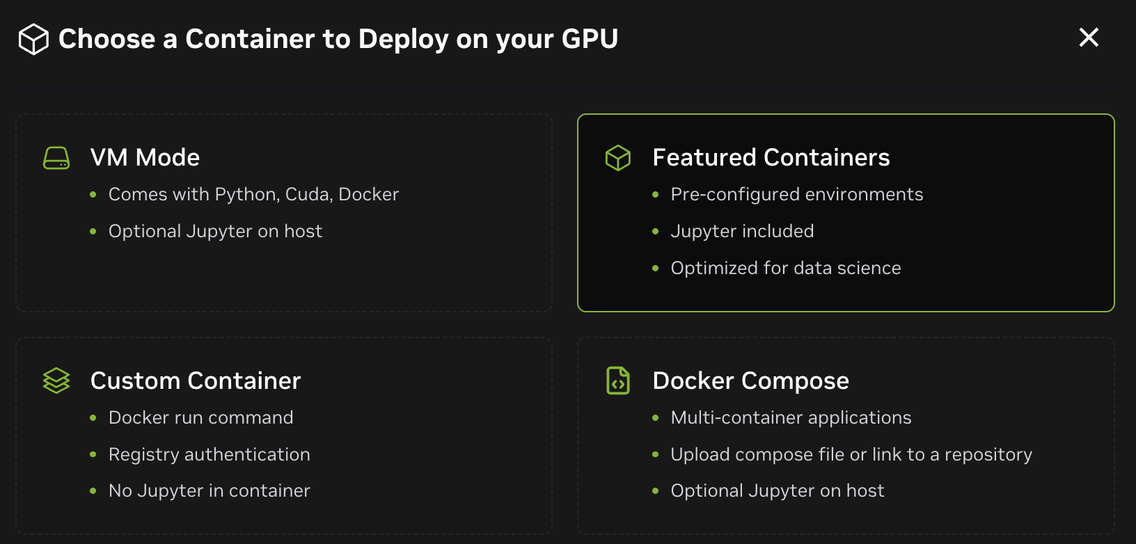
1. Attach the “NVIDIA RAPIDS” Container and choose “Apply”.
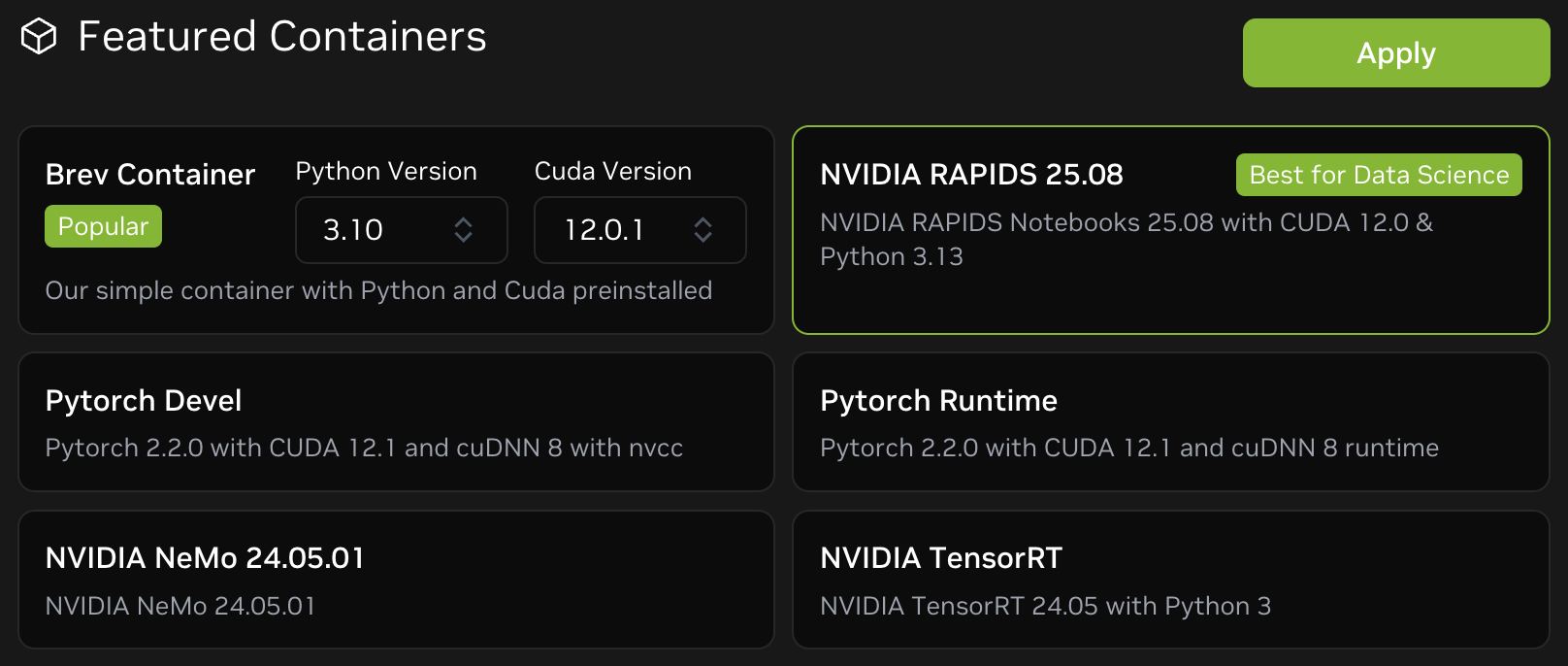
1. Give your instance a name and hit “Deploy”.
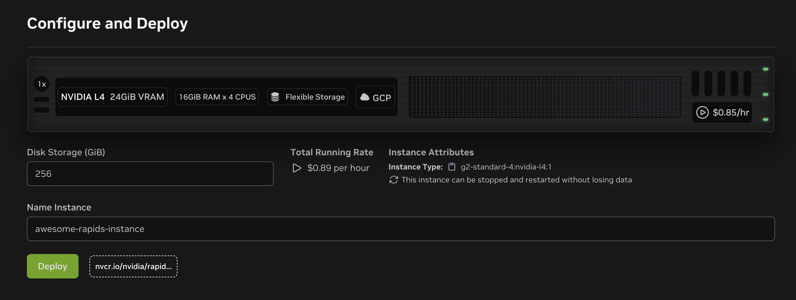
### Option 2. Setting up your Brev Launchable
Brev Launchables are shareable environment configurations that combine code, containers, and compute into a single
portable recipe. This option is most applicable if you want to set up a custom environment for a blueprint, like
our [Single-cell Analysis Blueprint](https://github.com/NVIDIA-AI-Blueprints/single-cell-analysis-blueprint/).
However, you can use this to create quick-start templates for many different kinds of projects when you want users to
drop into an environment that is ready to go (e.g. tutorials, workshops, demos, etc.).
You can read more about Brev Launchables in the [Getting Started Guide](https://docs.nvidia.com/brev/latest/launchables-getting-started.html).
1. Go to [Brev’s Launchable Creator](https://brev.nvidia.com/launchables/create) (requires account)
2. When asked **How would you like to provide your code files?**.
- Select “I have code files in a git repository”, and provide the link to a GitHub repository, if you have one that you’d like
to be mounted in the instance once is up.
- Otherwise, select “I don’t have any code files”.
3. When asked **What type of runtime environment do you need?** select “With container(s)”, and proceed.
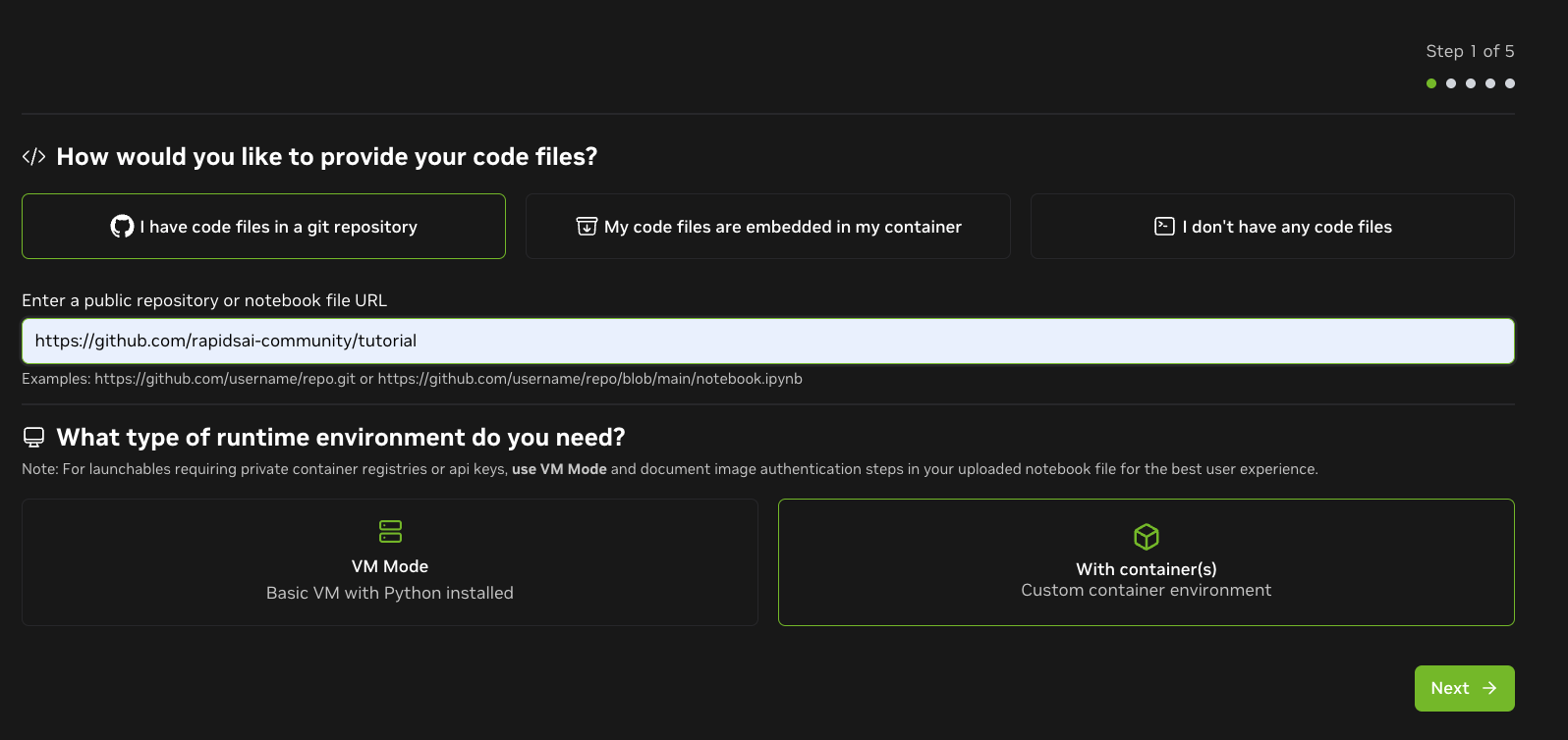
1. When prompted to **Choose a Container Configuration**, you have two options:
1. **“Featured Container”** and select the “NVIDIA RAPIDS” container: For a ready to go environment with the
entire RAPIDS stack and Jupyter configured.
- Select your desired compute environment. Make sure you select sufficient disk size to download the datasets you
want to work with. Note, you will not be able to resize the instance once created.
- Create a name for your launchable, and deploy.
2. **Docker Compose**: For a custom container that you can tailor to your needs.
- You can provide a `docker-compose.yaml` via url o from a local file. In the following template, make sure to
replace `` in the `volumes` path, with the name of your repository if you have one. Otherwise,
remove the `volumes`entry.
```yaml
services:
backend:
image: "rapidsai/notebooks:25.12a-cuda12-py3.13"
pull_policy: always
ulimits:
memlock: -1
stack: 67108864
shm_size: 1g
deploy:
resources:
reservations:
devices:
- driver: nvidia
count: all
capabilities: [gpu]
environment:
EXTRA_CONDA_PACKAGES: "hdbscan>=0.8.39 umap-learn>=0.5.7" # example of packages
ports:
- "8888:8888" # Expose JupyterLab
volumes:
- /home/ubuntu/:/notebooks/ # e.g tutorial if repo at https://github.com/rapidsai-community/tutorial
user: root
working_dir: /notebooks
entrypoint: ["/home/rapids/entrypoint.sh"]
command: python -m jupyter lab --allow-root --ip=0.0.0.0 --no-browser --NotebookApp.token='' --NotebookApp.password='' --notebook-dir=/notebooks
restart: unless-stopped
```
- Click “Validate”.
- Select your desired compute environment. Make sure you select sufficient disk size to download the datasets you
want to work with. Note, you will not be able to resize the instance once created.
- On the next page, when asked **Do you want a Jupyter Notebook experience?** select **No, I don’t want Jupyter**. This
is because the RAPIDS notebook container already have Jupyter setup. For convenience name the Secure Link to jupyter.
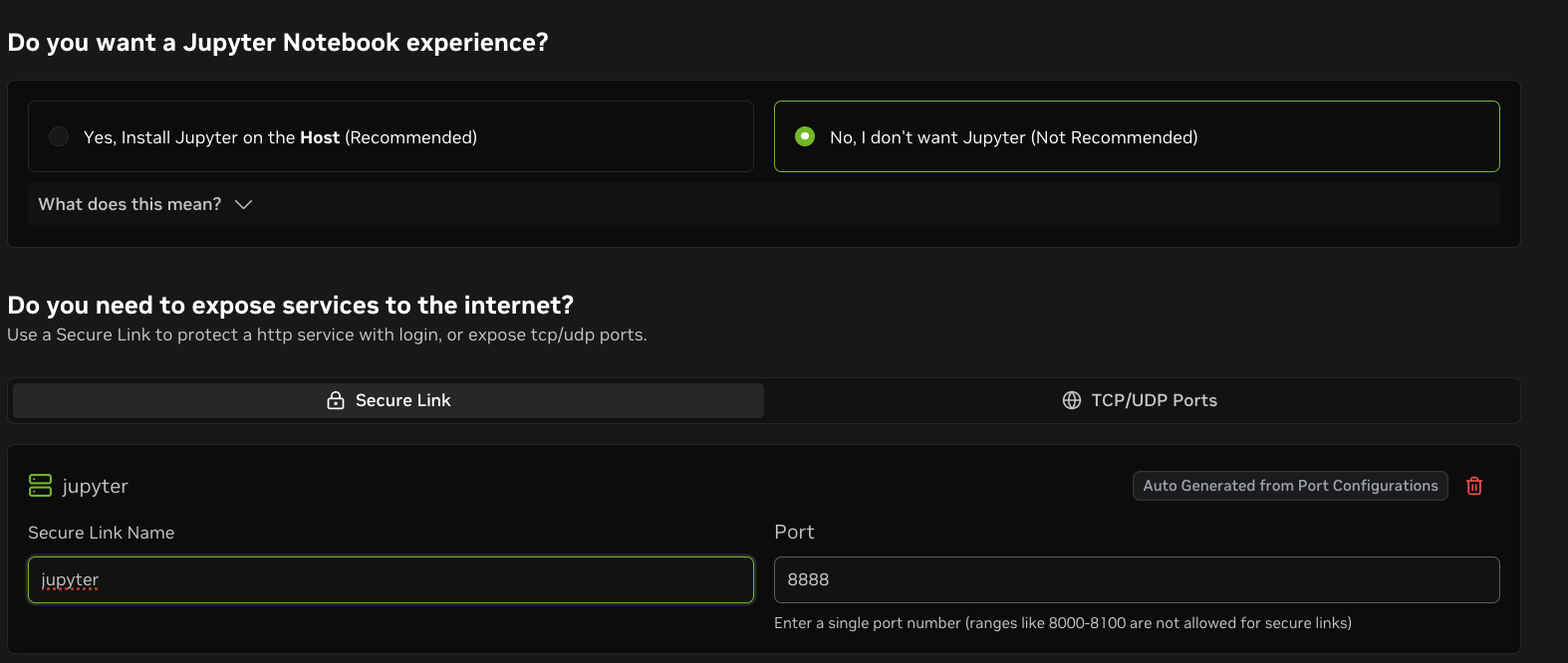
- Create a name for your launchable, and deploy.
## Accessing your instance
There are a few ways to access your instance:
1. Directly access Jupyter Lab from the Brev GUI
2. Using the Brev CLI to connect to your instance….
3. Using Visual Studio Code
4. Using SSH via your terminal
5. Access using the Brev tunnel
6. Sharing a service with others
### 1. Jupyter Notebook
To create and use a Jupyter Notebook, click “Open Notebook” at the top right after the page has deployed.
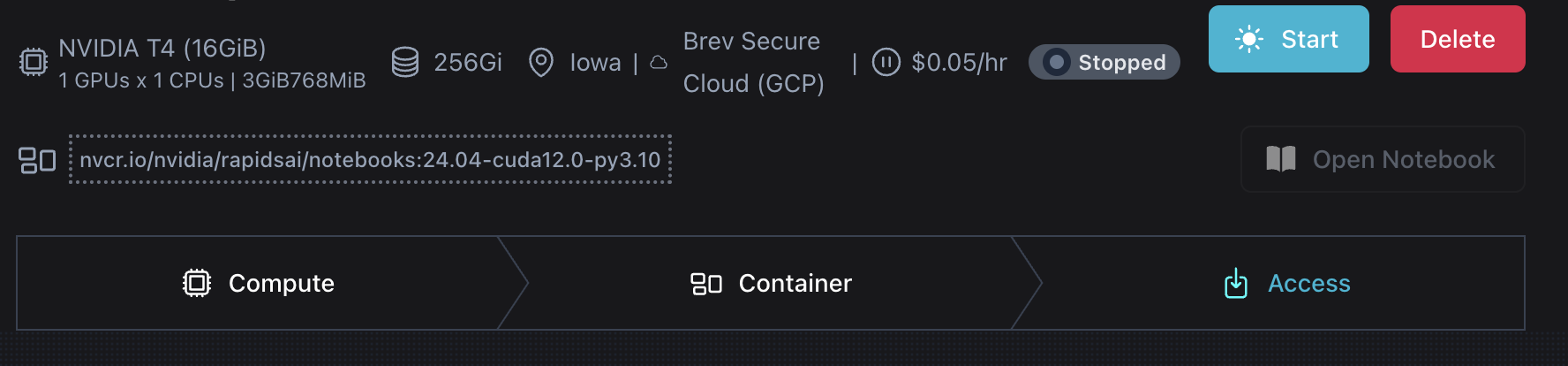
### 2. Brev CLI Install
If you want to access your launched Brev instance(s) via Visual Studio Code or SSH using terminal, you need to install the [Brev CLI according to these instructions](https://docs.nvidia.com/brev/latest/brev-cli.html) or this code below:
```bash
$ sudo bash -c "$(curl -fsSL https://raw.githubusercontent.com/brevdev/brev-cli/main/bin/install-latest.sh)" && brev login
```
#### 2.1 Brev CLI using Visual Studio Code
To connect to your Brev instance from VS Code open a new VS Code window and run:
```bash
$ brev open
```
It will automatically open a new VS Code window for you to use with RAPIDS.
#### 2.2 Brev CLI using SSH via your Terminal
To access your Brev instance from the terminal run:
```bash
$ brev shell
```
##### Forwarding a Port Locally
Assuming your Jupyter Notebook is running on port `8888` in your Brev environment, you can forward this port to your local machine using the following SSH command:
```bash
$ ssh -L 8888:localhost:8888 @ -p 22
```
This command forwards port `8888` on your local machine to port `8888` on the remote Brev environment.
Or for port `2222` (default port).
```bash
$ ssh @ -p 2222
```
Replace `username` with your username and `ip` with the ip listed if it’s different.
##### Accessing the Service
After running the command, open your web browser and navigate to your local host. You will be able to access the Jupyter Notebook running in your Brev environment as if it were running locally.
#### 3. Access the Jupyter Notebook via the Tunnel
The “Deployments” section will show that your Jupyter Notebook is running on port `8888`, and it is accessible via a shareable URL Ex: `jupyter0-i55ymhsr8.brevlab.com`.
Click on the link or copy and paste the URL into your web browser’s address bar to access the Jupyter Notebook interface directly.
##### 4. Share the Service
If you want to share access to this service with others, you can click on the “Share a Service” button.
You can also manage access by clicking “Edit Access” to control who has the ability to use this service.
### Check that your notebook has GPU Capabilities
You can verify that you have your requested GPU by running the `nvidia-smi` command.
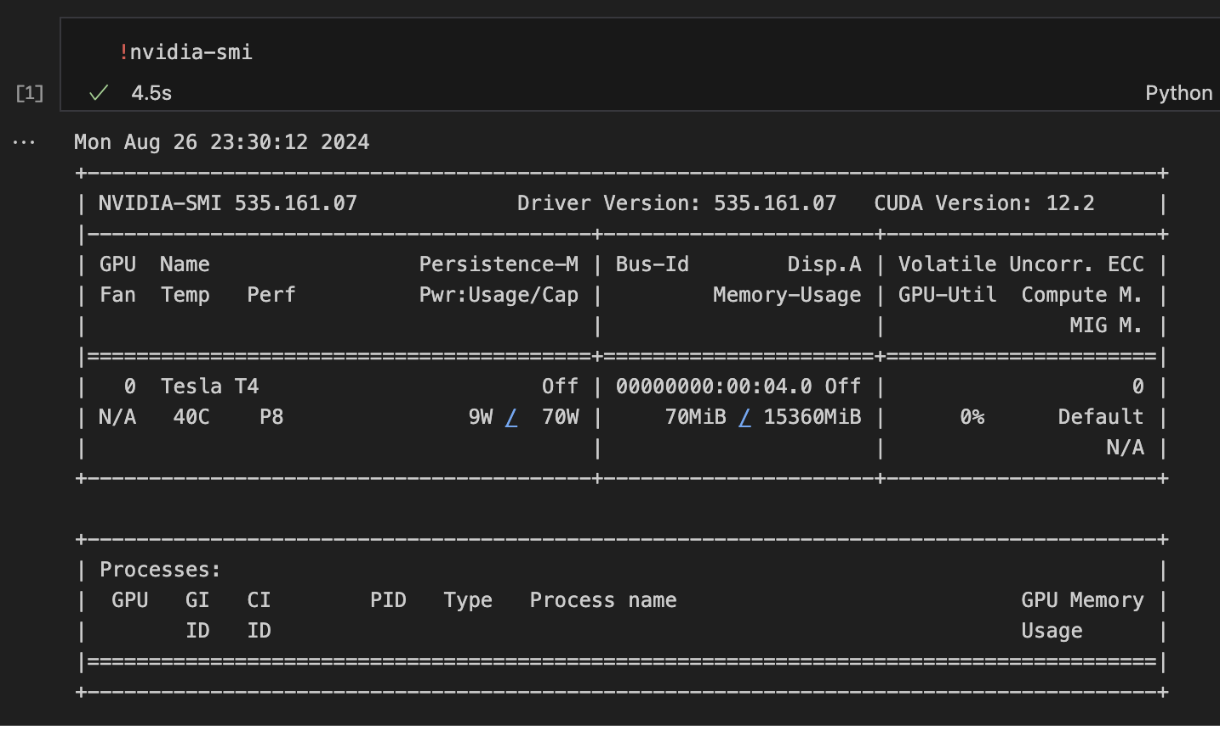
## Testing your RAPIDS Instance
You can verify your RAPIDS installation is working by importing `cudf` and creating a GPU dataframe.
```python
import cudf
gdf = cudf.DataFrame({"a": [1, 2, 3], "b": [4, 5, 6]})
print(gdf)
```
## Resources and tips
- [Brev Docs](https://brev.dev/)
- Please note: Git is not preinstalled in the RAPIDS container, but can be installed into the container when it is running using
```bash
$ apt update
```
```bash
$ apt install git -y
```
# index.html.md
Compute Engine Instance
Launch a Compute Engine instance and run RAPIDS.
single-node
Vertex AI
Launch the RAPIDS container in Vertex AI managed notebooks.
single-node
Google Kubernetes Engine (GKE)
Launch a RAPIDS cluster on managed Kubernetes.
multi-node
Dataproc
Launch a RAPIDS cluster on Dataproc.
multi-node
# index.html.md
IBM Virtual Server
Launch a virtual server and run RAPIDS.
single-node
# index.html.md
GitHub Actions
Run tests in GitHub Actions that depend on RAPIDS and NVIDIA GPUs.
single-node
# index.html.md
Azure Virtual Machine
Launch an Azure VM instance and run RAPIDS.
single-node
Azure Kubernetes Service (AKS)
Launch a RAPIDS cluster on managed Kubernetes.
multi-node
Azure Cluster via Dask
Launch a RAPIDS cluster on Azure VMs or Azure ML with Dask.
multi-node
Azure Machine Learning (Azure ML)
Launch RAPIDS Experiment on Azure ML.
single-node
multi-node
# index.html.md
Elastic Compute Cloud (EC2)
Launch an EC2 instance and run RAPIDS.
single-node
EC2 Cluster (with Dask)
Launch a RAPIDS cluster on EC2 with Dask.
multi-node
Elastic Kubernetes Service (EKS)
Launch a RAPIDS cluster on managed Kubernetes.
multi-node
Elastic Container Service (ECS)
Launch a RAPIDS cluster on managed container service.
multi-node
Sagemaker
Launch the RAPIDS container as a Sagemaker notebook.
single-node
multi-node
# index.html.md
Brev.dev
Deploy and run RAPIDS on NVIDIA Brev
single-node
# index.html.md
# GitHub Actions
GitHub Actions is a popular way to automatically run tests against code hosted on GitHub.
GitHub’s free tier includes basic runners (the machines that will run your code) and the paid tier includes support for [hosted runners with NVIDIA GPUs](https://github.blog/changelog/2024-07-08-github-actions-gpu-hosted-runners-are-now-generally-available/). This allows GPU specific code to be exercised as part of a CI workflow.
## Cost
As GPU runners are not included in the free tier projects will have to pay for GPU CI resources. Typically GPU runners cost a few cents per minute, check out the [GitHub documentation](https://docs.github.com/en/billing/managing-billing-for-github-actions/about-billing-for-github-actions#per-minute-rates-for-gpu-powered-larger-runners) for more information.
We recommend that projects set a [spending limit](https://docs.github.com/en/billing/managing-billing-for-github-actions/about-billing-for-github-actions#about-spending-limits) on their account/organization. That way your monthly bill will never be a surprise.
We also recommend that you only run GPU CI intentionally rather than on every pull request from every contributor. Check out the best practices section for more information.
## Getting started
### Setting up your GPU runners
First you’ll need to set up a way to pay GitHub. You can do this by [adding a payment method](https://docs.github.com/en/billing/managing-your-github-billing-settings/adding-or-editing-a-payment-method) to your organisation.
While you’re in your billing settings you should also decide what the maximum is that you wish to spend on GPU CI functionality and then set a [spending limit](https://docs.github.com/en/billing/managing-billing-for-github-actions/managing-your-spending-limit-for-github-actions) on your account.
Next you can go into the GitHub Actions settings for your account and configure a [larger runner](https://docs.github.com/en/actions/using-github-hosted-runners/using-larger-runners/about-larger-runners). You can find this settings page by visiting `https://github.com/organizations//settings/actions/runners`.
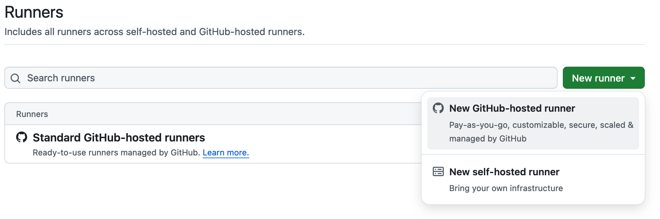
Next you need to give your runner a name, for example `linux-nvidia-gpu`, you’ll need to remember this for configuring your workflows later. Then you need to choose your runner settings:
- Under “Platform” select “Linux x64”
- Under “Image” switch to the “Partner” tab and choose “NVIDIA GPU-Optimized Image for AI and HPC”
- Under “Size” switch to the “GPU-powered” tab and select your preferred NVIDIA hardware
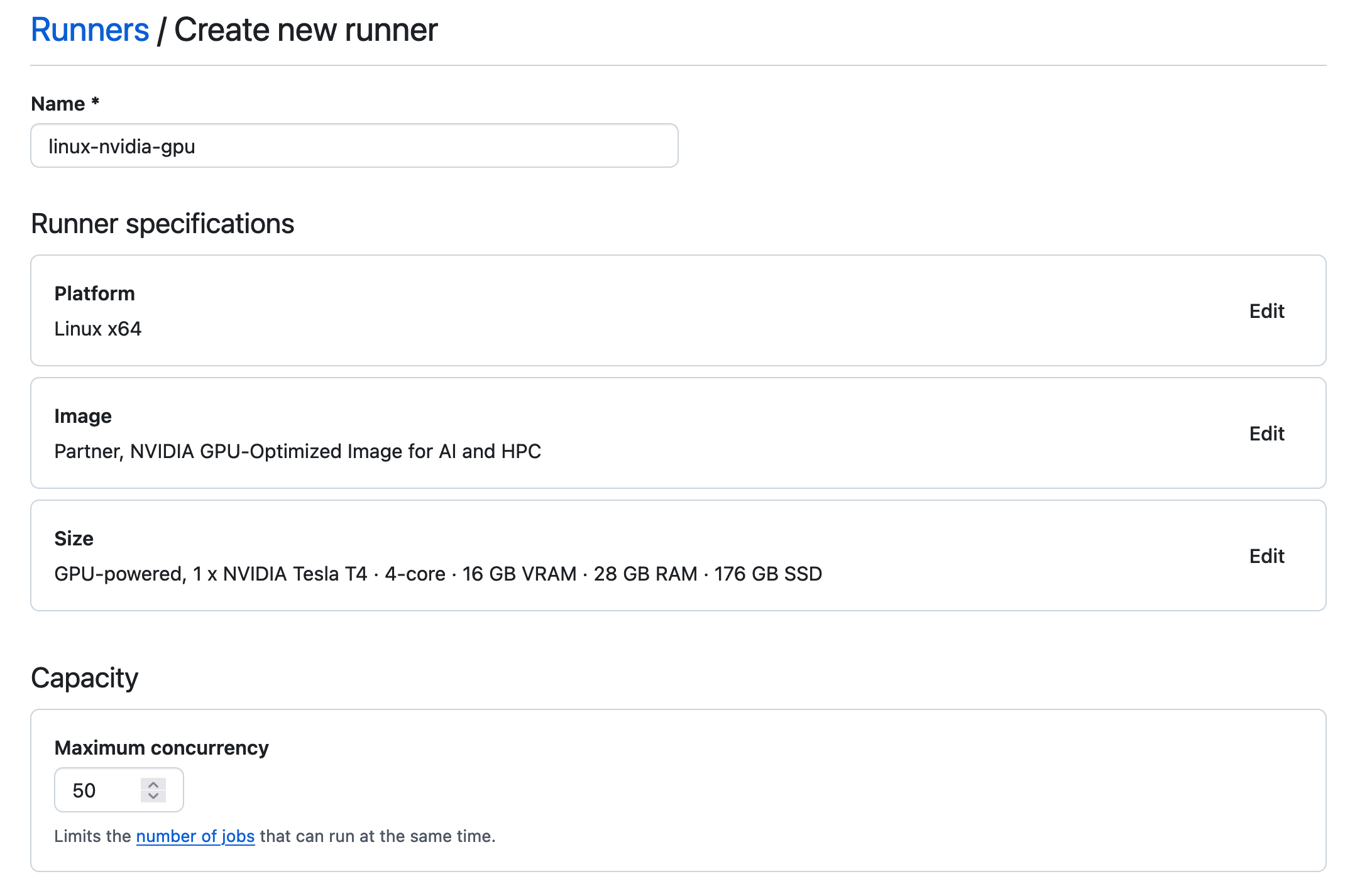
Then set your preferred maximum concurrency and then choose “Create runner”.
### Configuring your workflows
To configure your workflow to use your new GPU runners you need to set the `runs-on` property to match the name you gave the runner group.
```yaml
name: GitHub Actions GPU Demo
run-name: ${{ github.actor }} is testing out GPU GitHub Actions 🚀
on: [push]
jobs:
gpu-workflow:
runs-on: linux-nvidia-gpu
steps:
- name: Check GPU is available
run: nvidia-smi
```
## Best practices
Adding GitHub Actions runners to your project that cost money requires you to put some extra thought into when you want those workflows to run. Setting a spending cap allows you to keep control of how much you are spending, but you still want to get the most for your money. Here are some tips on when to effectively use GPU runners in your projects.
### Use labels to trigger workloads
Instead of always triggering your GPU workflows on every push or pull request you can use labels to trigger workflows. This is a great option if your project is public and anyone can make a pull request with any arbitrary code. You may want to have a mechanism for a trusted maintainer or collaborator to trigger the GPU workflow manually.
The scikit-learn project solved this by having a label that triggers the workflow.
```yaml
name: NVIDIA GPU workflow
on:
pull_request:
types:
- labeled
jobs:
tests:
if: contains(github.event.pull_request.labels.*.name, 'GPU CI')
runs-on:
group: linux-nvidia-gpu
steps: ...
```
The above config specifies a workflow should only be run when the `GPU CI` label is added to the pull request. They then have a second [label remover workflow](https://github.com/scikit-learn/scikit-learn/blob/9d39f57399d6f1f7d8e8d4351dbc3e9244b98d28/.github/workflows/cuda-label-remover.yml) which removed the label again, which allows a maintainer to add it again in the future to trigger the GPU CI workflow any number of times during the review of the pull request.
### Run nightly
Some projects might not need to run GPU tests for every pull request, but instead might prefer to run a nightly regression test to ensure that nothing that has been merged has broken GPU functionality.
You can configure a GitHub Actions workflow to run on a schedule and use [an action](https://github.com/marketplace/actions/failed-build-issue) to open an issue if the workflow fails.
```yaml
name: Nightly GPU Tests
on:
schedule:
- cron: "0 0 * * *" # Run every day at 00:00 UTC
jobs:
tests:
name: GPU Tests
runs-on: linux-nvidia-gpu
steps:
- uses: actions/checkout@v4
- name: Run tests
run: |
# Run tests here
- name: Notify failed build
uses: jayqi/failed-build-issue-action@v1
if: failure() && github.event.pull_request == null
with:
github-token: ${{ secrets.GITHUB_TOKEN }}
```
### Run only on certain codepaths
You may also want to only run your GPU CI tests when code at certain paths has been modified. To do this you can use the [`on.push.paths` filter](https://docs.github.com/en/actions/writing-workflows/workflow-syntax-for-github-actions#example-including-paths).
```yaml
name: GPU Tests
on:
push:
paths:
- "src/gpu_submodule/**/*.py"
jobs:
tests:
name: GPU Tests
runs-on: linux-nvidia-gpu
steps: ...
```
## Further Reading
- [Blog from scikit-learn Developers on their experiences](https://betatim.github.io/posts/github-action-with-gpu/)
# index.html.md
# Continuous Integration
GitHub Actions
Run tests in GitHub Actions that depend on RAPIDS and NVIDIA GPUs.
single-node
# index.html.md
# How to Setup InfiniBand on Azure
[Azure GPU optimized virtual machines](https://learn.microsoft.com/en-us/azure/virtual-machines/sizes-gpu) provide
a low latency and high bandwidth InfiniBand network. This guide walks through the steps to enable InfiniBand to
optimize network performance.
## Build a Virtual Machine
Start by creating a GPU optimized VM from the Azure portal. Below is an example that we will use
for demonstration.
- Create new VM instance.
- Select `East US` region.
- Change `Availability options` to `Availability set` and create a set.
- If building multiple instances put additional instances in the same set.
- Use the 2nd Gen Ubuntu 24.04 image.
- Search all images for `Ubuntu Server 24.04` and choose the second one down on the list.
- Change size to `ND40rs_v2`.
- Set password login with credentials.
- User `someuser`
- Password `somepassword`
- Leave all other options as default.
Then connect to the VM using your preferred method.
## Install Software
Before installing the drivers ensure the system is up to date.
```shell
sudo apt-get update
sudo apt-get upgrade -y
```
### NVIDIA Drivers
The commands below should work for Ubuntu. See the [CUDA Toolkit documentation](https://docs.nvidia.com/cuda/index.html#installation-guides) for details on installing on other operating systems.
```shell
sudo apt-get install -y linux-headers-$(uname -r)
distribution=$(. /etc/os-release;echo $ID$VERSION_ID | sed -e 's/\.//g')
wget https://developer.download.nvidia.com/compute/cuda/repos/$distribution/x86_64/cuda-keyring_1.1-1_all.deb
sudo dpkg -i cuda-keyring_1.1-1_all.deb
sudo apt-get update
sudo apt-get -y install cuda-drivers
```
Restart VM instance
```shell
sudo reboot
```
Once the VM boots, reconnect and run `nvidia-smi` to verify driver installation.
```shell
nvidia-smi
```
```shell
Mon Nov 14 20:32:39 2022
+-----------------------------------------------------------------------------+
| NVIDIA-SMI 520.61.05 Driver Version: 520.61.05 CUDA Version: 11.8 |
|-------------------------------+----------------------+----------------------+
| GPU Name Persistence-M| Bus-Id Disp.A | Volatile Uncorr. ECC |
| Fan Temp Perf Pwr:Usage/Cap| Memory-Usage | GPU-Util Compute M. |
| | | MIG M. |
|===============================+======================+======================|
| 0 Tesla V100-SXM2... On | 00000001:00:00.0 Off | 0 |
| N/A 34C P0 41W / 300W | 445MiB / 32768MiB | 0% Default |
| | | N/A |
+-------------------------------+----------------------+----------------------+
| 1 Tesla V100-SXM2... On | 00000002:00:00.0 Off | 0 |
| N/A 37C P0 43W / 300W | 4MiB / 32768MiB | 0% Default |
| | | N/A |
+-------------------------------+----------------------+----------------------+
| 2 Tesla V100-SXM2... On | 00000003:00:00.0 Off | 0 |
| N/A 34C P0 42W / 300W | 4MiB / 32768MiB | 0% Default |
| | | N/A |
+-------------------------------+----------------------+----------------------+
| 3 Tesla V100-SXM2... On | 00000004:00:00.0 Off | 0 |
| N/A 35C P0 44W / 300W | 4MiB / 32768MiB | 0% Default |
| | | N/A |
+-------------------------------+----------------------+----------------------+
| 4 Tesla V100-SXM2... On | 00000005:00:00.0 Off | 0 |
| N/A 35C P0 41W / 300W | 4MiB / 32768MiB | 0% Default |
| | | N/A |
+-------------------------------+----------------------+----------------------+
| 5 Tesla V100-SXM2... On | 00000006:00:00.0 Off | 0 |
| N/A 36C P0 43W / 300W | 4MiB / 32768MiB | 0% Default |
| | | N/A |
+-------------------------------+----------------------+----------------------+
| 6 Tesla V100-SXM2... On | 00000007:00:00.0 Off | 0 |
| N/A 37C P0 44W / 300W | 4MiB / 32768MiB | 0% Default |
| | | N/A |
+-------------------------------+----------------------+----------------------+
| 7 Tesla V100-SXM2... On | 00000008:00:00.0 Off | 0 |
| N/A 38C P0 44W / 300W | 4MiB / 32768MiB | 0% Default |
| | | N/A |
+-------------------------------+----------------------+----------------------+
+-----------------------------------------------------------------------------+
| Processes: |
| GPU GI CI PID Type Process name GPU Memory |
| ID ID Usage |
|=============================================================================|
| 0 N/A N/A 1396 G /usr/lib/xorg/Xorg 427MiB |
| 0 N/A N/A 1762 G /usr/bin/gnome-shell 16MiB |
| 1 N/A N/A 1396 G /usr/lib/xorg/Xorg 4MiB |
| 2 N/A N/A 1396 G /usr/lib/xorg/Xorg 4MiB |
| 3 N/A N/A 1396 G /usr/lib/xorg/Xorg 4MiB |
| 4 N/A N/A 1396 G /usr/lib/xorg/Xorg 4MiB |
| 5 N/A N/A 1396 G /usr/lib/xorg/Xorg 4MiB |
| 6 N/A N/A 1396 G /usr/lib/xorg/Xorg 4MiB |
| 7 N/A N/A 1396 G /usr/lib/xorg/Xorg 4MiB |
+-----------------------------------------------------------------------------+
```
### InfiniBand Driver
On Ubuntu 24.04
```shell
sudo apt-get install -y automake dh-make git libcap2 libnuma-dev libtool make pkg-config udev curl librdmacm-dev rdma-core \
libgfortran5 bison chrpath flex graphviz gfortran tk quilt swig tcl ibverbs-utils
```
Check install
```shell
ibv_devinfo
```
```shell
hca_id: mlx5_0
transport: InfiniBand (0)
fw_ver: 16.28.4000
node_guid: 0015:5dff:fe33:ff2c
sys_image_guid: 0c42:a103:00b3:2f68
vendor_id: 0x02c9
vendor_part_id: 4120
hw_ver: 0x0
board_id: MT_0000000010
phys_port_cnt: 1
port: 1
state: PORT_ACTIVE (4)
max_mtu: 4096 (5)
active_mtu: 4096 (5)
sm_lid: 7
port_lid: 115
port_lmc: 0x00
link_layer: InfiniBand
hca_id: rdmaP36305p0s2
transport: InfiniBand (0)
fw_ver: 2.43.7008
node_guid: 6045:bdff:feed:8445
sys_image_guid: 043f:7203:0003:d583
vendor_id: 0x02c9
vendor_part_id: 4100
hw_ver: 0x0
board_id: MT_1090111019
phys_port_cnt: 1
port: 1
state: PORT_ACTIVE (4)
max_mtu: 4096 (5)
active_mtu: 1024 (3)
sm_lid: 0
port_lid: 0
port_lmc: 0x00
link_layer: Ethernet
```
#### Enable IPoIB
```shell
sudo sed -i -e 's/# OS.EnableRDMA=y/OS.EnableRDMA=y/g' /etc/waagent.conf
```
Reboot and reconnect.
```shell
sudo reboot
```
#### Check IB
```shell
ip addr show
```
```shell
1: lo: mtu 65536 qdisc noqueue state UNKNOWN group default qlen 1000
link/loopback 00:00:00:00:00:00 brd 00:00:00:00:00:00
inet 127.0.0.1/8 scope host lo
valid_lft forever preferred_lft forever
inet6 ::1/128 scope host
valid_lft forever preferred_lft forever
2: eth0: mtu 1500 qdisc mq state UP group default qlen 1000
link/ether 60:45:bd:a7:42:cc brd ff:ff:ff:ff:ff:ff
inet 10.6.0.5/24 brd 10.6.0.255 scope global eth0
valid_lft forever preferred_lft forever
inet6 fe80::6245:bdff:fea7:42cc/64 scope link
valid_lft forever preferred_lft forever
3: eth1: mtu 1500 qdisc noop state DOWN group default qlen 1000
link/ether 00:15:5d:33:ff:16 brd ff:ff:ff:ff:ff:ff
4: enP44906s1: mtu 1500 qdisc mq master eth0 state UP group default qlen 1000
link/ether 60:45:bd:a7:42:cc brd ff:ff:ff:ff:ff:ff
altname enP44906p0s2
5: ibP59423s2: mtu 4092 qdisc noop state DOWN group default qlen 256
link/infiniband 00:00:09:27:fe:80:00:00:00:00:00:00:00:15:5d:ff:fd:33:ff:16 brd 00:ff:ff:ff:ff:12:40:1b:80:1d:00:00:00:00:00:00:ff:ff:ff:ff
altname ibP59423p0s2
```
```shell
nvidia-smi topo -m
```
```shell
GPU0 GPU1 GPU2 GPU3 GPU4 GPU5 GPU6 GPU7 mlx5_0 CPU Affinity NUMA Affinity
GPU0 X NV2 NV1 NV2 NODE NODE NV1 NODE NODE 0-19 0
GPU1 NV2 X NV2 NV1 NODE NODE NODE NV1 NODE 0-19 0
GPU2 NV1 NV2 X NV1 NV2 NODE NODE NODE NODE 0-19 0
GPU3 NV2 NV1 NV1 X NODE NV2 NODE NODE NODE 0-19 0
GPU4 NODE NODE NV2 NODE X NV1 NV1 NV2 NODE 0-19 0
GPU5 NODE NODE NODE NV2 NV1 X NV2 NV1 NODE 0-19 0
GPU6 NV1 NODE NODE NODE NV1 NV2 X NV2 NODE 0-19 0
GPU7 NODE NV1 NODE NODE NV2 NV1 NV2 X NODE 0-19 0
mlx5_0 NODE NODE NODE NODE NODE NODE NODE NODE X
Legend:
X = Self
SYS = Connection traversing PCIe as well as the SMP interconnect between NUMA nodes (e.g., QPI/UPI)
NODE = Connection traversing PCIe as well as the interconnect between PCIe Host Bridges within a NUMA node
PHB = Connection traversing PCIe as well as a PCIe Host Bridge (typically the CPU)
PXB = Connection traversing multiple PCIe bridges (without traversing the PCIe Host Bridge)
PIX = Connection traversing at most a single PCIe bridge
NV# = Connection traversing a bonded set of # NVLinks
```
### Install UCXX and tools
```shell
wget https://github.com/conda-forge/miniforge/releases/latest/download/Mambaforge-Linux-x86_64.sh
bash Mambaforge-Linux-x86_64.sh
```
Accept the default and allow conda init to run.
```shell
~/mambaforge/bin/conda init
```
Then start a new shell.
Create a conda environment (see [UCXX](https://docs.rapids.ai/api/ucxx/nightly/install/) docs)
```shell
mamba create -n ucxx -c rapidsai-nightly -c conda-forge -c nvidia rapids=25.12 python=3.13 'cuda-version>=12.0,<=12.9' ipython dask distributed distributed-ucxx numpy cupy pytest pynvml -y
mamba activate ucxx
```
Clone UCXX repo locally
```shell
git clone https://github.com/rapidsai/ucxx.git
cd ucxx
```
### Run Tests
Start by running the UCXX test suite, from within the `ucxx` repo:
```shell
pytest -vs python/ucxx/ucxx/_lib/tests
pytest -vs python/ucxx/ucxx/_lib_async/tests
```
Now check to see if InfiniBand works, for that you can run some of the benchmarks that we include in UCXX, for example:
```shell
# cd out of the ucxx directory
cd ..
# Let UCX pick the best transport (expecting NVLink when available,
# otherwise InfiniBand, or TCP in worst case) on devices 0 and 1
python -m ucxx.benchmarks.send_recv --server-dev 0 --client-dev 1 -o rmm --reuse-alloc -n 128MiB
# Force TCP-only on devices 0 and 1
UCX_TLS=tcp,cuda_copy python -m ucxx.benchmarks.send_recv --server-dev 0 --client-dev 1 -o rmm --reuse-alloc -n 128MiB
```
We expect the first case above to have much higher bandwidth than the second. If you happen to have both
NVLink and InfiniBand connectivity, then you may limit to the specific transport by specifying `UCX_TLS`, e.g.:
```shell
# NVLink (if available) or TCP
UCX_TLS=tcp,cuda_copy,cuda_ipc
# InfiniBand (if available) or TCP
UCX_TLS=tcp,cuda_copy,rc
```
## Run Benchmarks
Finally, let’s run the [merge benchmark](https://github.com/rapidsai/dask-cuda/blob/HEAD/dask_cuda/benchmarks/local_cudf_merge.py) from `dask-cuda`.
This benchmark uses Dask to perform a merge of two dataframes that are distributed across all the available GPUs on your
VM. Merges are a challenging benchmark in a distributed setting since they require communication-intensive shuffle
operations of the participating dataframes
(see the [Dask documentation](https://docs.dask.org/en/stable/dataframe-best-practices.html#avoid-full-data-shuffling)
for more on this type of operation). To perform the merge, each dataframe is shuffled such that rows with the same join
key appear on the same GPU. This results in an [all-to-all](https://en.wikipedia.org/wiki/All-to-all_(parallel_pattern))
communication pattern which requires a lot of communication between the GPUs. As a result, network
performance will be very important for the throughput of the benchmark.
Below we are running for devices 0 through 7 (inclusive), you will want to adjust that for the number of devices available on your VM, the default
is to run on GPU 0 only. Additionally, `--chunk-size 100_000_000` is a safe value for 32GB GPUs, you may
adjust that proportional to the size of the GPU you have (it scales linearly, so `50_000_000` should
be good for 16GB or `150_000_000` for 48GB).
```shell
# Default Dask TCP communication protocol
python -m dask_cuda.benchmarks.local_cudf_merge --devs 0,1,2,3,4,5,6,7 --chunk-size 100_000_000 --no-show-p2p-bandwidth
```
```shell
Merge benchmark
--------------------------------------------------------------------------------
Backend | dask
Merge type | gpu
Rows-per-chunk | 100000000
Base-chunks | 8
Other-chunks | 8
Broadcast | default
Protocol | tcp
Device(s) | 0,1,2,3,4,5,6,7
RMM Pool | True
Frac-match | 0.3
Worker thread(s) | 1
Data processed | 23.84 GiB
Number of workers | 8
================================================================================
Wall clock | Throughput
--------------------------------------------------------------------------------
48.51 s | 503.25 MiB/s
47.85 s | 510.23 MiB/s
41.20 s | 592.57 MiB/s
================================================================================
Throughput | 532.43 MiB/s +/- 22.13 MiB/s
Bandwidth | 44.76 MiB/s +/- 0.93 MiB/s
Wall clock | 45.85 s +/- 3.30 s
```
```shell
# UCX protocol
python -m dask_cuda.benchmarks.local_cudf_merge --devs 0,1,2,3,4,5,6,7 --chunk-size 100_000_000 --protocol ucx --no-show-p2p-bandwidth
```
```shell
Merge benchmark
--------------------------------------------------------------------------------
Backend | dask
Merge type | gpu
Rows-per-chunk | 100000000
Base-chunks | 8
Other-chunks | 8
Broadcast | default
Protocol | ucx
Device(s) | 0,1,2,3,4,5,6,7
RMM Pool | True
Frac-match | 0.3
TCP | None
InfiniBand | None
NVLink | None
Worker thread(s) | 1
Data processed | 23.84 GiB
Number of workers | 8
================================================================================
Wall clock | Throughput
--------------------------------------------------------------------------------
9.57 s | 2.49 GiB/s
6.01 s | 3.96 GiB/s
9.80 s | 2.43 GiB/s
================================================================================
Throughput | 2.82 GiB/s +/- 341.13 MiB/s
Bandwidth | 159.89 MiB/s +/- 8.96 MiB/s
Wall clock | 8.46 s +/- 1.73 s
```
# index.html.md
# Dask Operator
Many libraries in RAPIDS can leverage Dask to scale out computation onto multiple GPUs and multiple nodes.
[Dask has an operator for Kubernetes](https://kubernetes.dask.org/en/latest/) which allows you to launch Dask clusters as native Kubernetes resources.
With the operator and associated Custom Resource Definitions (CRDs)
you can create `DaskCluster`, `DaskWorkerGroup` and `DaskJob` resources that describe your Dask components and the operator will
create the appropriate Kubernetes resources like `Pods` and `Services` to launch the cluster.
## Installation
Your Kubernetes cluster must have GPU nodes and have [up to date NVIDIA drivers installed](https://docs.nvidia.com/datacenter/cloud-native/gpu-operator/getting-started.html).
To install the Dask operator follow the [instructions in the Dask documentation](https://kubernetes.dask.org/en/latest/installing.html).
## Configuring a RAPIDS `DaskCluster`
To configure the `DaskCluster` resource to run RAPIDS you need to set a few things:
- The container image must contain RAPIDS, the [official RAPIDS container images](https://docs.rapids.ai/install/#docker) are a good choice for this.
- The Dask workers must be configured with one or more NVIDIA GPU resources.
- The worker command must be set to `dask-cuda-worker`.
## Example using `kubectl`
Here is an example resource manifest for launching a RAPIDS Dask cluster.
```yaml
# rapids-dask-cluster.yaml
apiVersion: kubernetes.dask.org/v1
kind: DaskCluster
metadata:
name: rapids-dask-cluster
labels:
dask.org/cluster-name: rapids-dask-cluster
spec:
worker:
replicas: 2
spec:
containers:
- name: worker
image: "rapidsai/base:25.12a-cuda12-py3.13"
imagePullPolicy: "IfNotPresent"
args:
- dask-cuda-worker
- --name
- $(DASK_WORKER_NAME)
resources:
limits:
nvidia.com/gpu: "1"
scheduler:
spec:
containers:
- name: scheduler
image: "rapidsai/base:25.12a-cuda12-py3.13"
imagePullPolicy: "IfNotPresent"
env:
args:
- dask-scheduler
ports:
- name: tcp-comm
containerPort: 8786
protocol: TCP
- name: http-dashboard
containerPort: 8787
protocol: TCP
readinessProbe:
httpGet:
port: http-dashboard
path: /health
initialDelaySeconds: 5
periodSeconds: 10
livenessProbe:
httpGet:
port: http-dashboard
path: /health
initialDelaySeconds: 15
periodSeconds: 20
service:
type: ClusterIP
selector:
dask.org/cluster-name: rapids-dask-cluster
dask.org/component: scheduler
ports:
- name: tcp-comm
protocol: TCP
port: 8786
targetPort: "tcp-comm"
- name: http-dashboard
protocol: TCP
port: 8787
targetPort: "http-dashboard"
```
You can create this cluster with `kubectl`.
```bash
$ kubectl apply -f rapids-dask-cluster.yaml
```
### Manifest breakdown
Let’s break this manifest down section by section.
#### Metadata
At the top we see the `DaskCluster` resource type and general metadata.
```yaml
apiVersion: kubernetes.dask.org/v1
kind: DaskCluster
metadata:
name: rapids-dask-cluster
labels:
dask.org/cluster-name: rapids-dask-cluster
spec:
worker:
# ...
scheduler:
# ...
```
Then inside the `spec` we have `worker` and `scheduler` sections.
#### Worker
The worker contains a `replicas` option to set how many workers you need and a `spec` that describes what each worker Pod should look like.
The spec is a nested [`Pod` spec](https://kubernetes.io/docs/concepts/workloads/pods/) that the operator will use when creating new `Pod` resources.
```yaml
# ...
spec:
worker:
replicas: 2
spec:
containers:
- name: worker
image: "rapidsai/base:25.12a-cuda12-py3.13"
imagePullPolicy: "IfNotPresent"
args:
- dask-cuda-worker
- --name
- $(DASK_WORKER_NAME)
resources:
limits:
nvidia.com/gpu: "1"
scheduler:
# ...
```
Inside our Pod spec we are configuring one container that uses the `rapidsai/base` container image.
It also sets the `args` to start the `dask-cuda-worker` and configures one NVIDIA GPU.
#### Scheduler
Next we have a `scheduler` section that also contains a `spec` for the scheduler Pod and a `service` which will be used by the operator to create a `Service` resource to expose the scheduler.
```yaml
# ...
spec:
worker:
# ...
scheduler:
spec:
containers:
- name: scheduler
image: "rapidsai/base:25.12a-cuda12-py3.13"
imagePullPolicy: "IfNotPresent"
args:
- dask-scheduler
ports:
- name: tcp-comm
containerPort: 8786
protocol: TCP
- name: http-dashboard
containerPort: 8787
protocol: TCP
readinessProbe:
httpGet:
port: http-dashboard
path: /health
initialDelaySeconds: 5
periodSeconds: 10
livenessProbe:
httpGet:
port: http-dashboard
path: /health
initialDelaySeconds: 15
periodSeconds: 20
service:
# ...
```
For the scheduler Pod we are also setting the `rapidsai/base` container image, mainly to ensure our Dask versions match between
the scheduler and workers. We ensure that the `dask-scheduler` command is configured.
Then we configure both the Dask communication port on `8786` and the Dask dashboard on `8787` and add some probes so that Kubernetes can monitor
the health of the scheduler.
#### NOTE
The ports must have the `tcp-` and `http-` prefixes if your Kubernetes cluster uses [Istio](https://istio.io/) to ensure the [Envoy proxy](https://www.envoyproxy.io/) doesn’t mangle the traffic.
Then we configure the `Service`.
```yaml
# ...
spec:
worker:
# ...
scheduler:
spec:
# ...
service:
type: ClusterIP
selector:
dask.org/cluster-name: rapids-dask-cluster
dask.org/component: scheduler
ports:
- name: tcp-comm
protocol: TCP
port: 8786
targetPort: "tcp-comm"
- name: http-dashboard
protocol: TCP
port: 8787
targetPort: "http-dashboard"
```
This example shows using a `ClusterIP` service which will not expose the Dask cluster outside of Kubernetes. If you prefer you could set this to
[`LoadBalancer`](https://kubernetes.io/docs/concepts/services-networking/service/#loadbalancer) or [`NodePort`](https://kubernetes.io/docs/concepts/services-networking/service/#type-nodeport) to make this externally accessible.
It has a `selector` that matches the scheduler Pod and the same ports configured.
### Accessing your Dask cluster
Once you have created your `DaskCluster` resource we can use `kubectl` to check the status of all the other resources it created for us.
```console
$ kubectl get all -l dask.org/cluster-name=rapids-dask-cluster
NAME READY STATUS RESTARTS AGE
pod/rapids-dask-cluster-default-worker-group-worker-0c202b85fd 1/1 Running 0 4m13s
pod/rapids-dask-cluster-default-worker-group-worker-ff5d376714 1/1 Running 0 4m13s
pod/rapids-dask-cluster-scheduler 1/1 Running 0 4m14s
NAME TYPE CLUSTER-IP EXTERNAL-IP PORT(S) AGE
service/rapids-dask-cluster-service ClusterIP 10.96.223.217 8786/TCP,8787/TCP 4m13s
```
Here you can see our scheduler Pod and two worker Pods along with the scheduler service.
If you have a Python session running within the Kubernetes cluster (like the [example one on the Kubernetes page](../../platforms/kubernetes.md)) you should be able
to connect a Dask distributed client directly.
```python
from dask.distributed import Client
client = Client("rapids-dask-cluster-scheduler:8786")
```
Alternatively if you are outside of the Kubernetes cluster you can change the `Service` to use [`LoadBalancer`](https://kubernetes.io/docs/concepts/services-networking/service/#loadbalancer) or [`NodePort`](https://kubernetes.io/docs/concepts/services-networking/service/#type-nodeport) or use `kubectl` to port forward the connection locally.
```console
$ kubectl port-forward svc/rapids-dask-cluster-service 8786:8786
Forwarding from 127.0.0.1:8786 -> 8786
```
```python
from dask.distributed import Client
client = Client("localhost:8786")
```
## Example using `KubeCluster`
In addition to creating clusters via `kubectl` you can also do so from Python with [`dask_kubernetes.operator.KubeCluster`](https://kubernetes.dask.org/en/latest/operator_kubecluster.html#dask_kubernetes.operator.KubeCluster). This class implements the Dask Cluster Manager interface and under the hood creates and manages the `DaskCluster` resource for you.
```python
from dask_kubernetes.operator import KubeCluster
cluster = KubeCluster(
name="rapids-dask",
image="rapidsai/base:25.12a-cuda12-py3.13",
n_workers=3,
resources={"limits": {"nvidia.com/gpu": "1"}},
worker_command="dask-cuda-worker",
)
```
If we check with `kubectl` we can see the above Python generated the same `DaskCluster` resource as the `kubectl` example above.
```console
$ kubectl get daskclusters
NAME AGE
rapids-dask-cluster 3m28s
$ kubectl get all -l dask.org/cluster-name=rapids-dask-cluster
NAME READY STATUS RESTARTS AGE
pod/rapids-dask-cluster-default-worker-group-worker-07d674589a 1/1 Running 0 3m30s
pod/rapids-dask-cluster-default-worker-group-worker-a55ed88265 1/1 Running 0 3m30s
pod/rapids-dask-cluster-default-worker-group-worker-df785ab050 1/1 Running 0 3m30s
pod/rapids-dask-cluster-scheduler 1/1 Running 0 3m30s
NAME TYPE CLUSTER-IP EXTERNAL-IP PORT(S) AGE
service/rapids-dask-cluster-service ClusterIP 10.96.200.202 8786/TCP,8787/TCP 3m30s
```
With this cluster object in Python we can also connect a client to it directly without needing to know the address as Dask will discover that for us. It also automatically sets up port forwarding if you are outside of the Kubernetes cluster.
```python
from dask.distributed import Client
client = Client(cluster)
```
This object can also be used to scale the workers up and down.
```python
cluster.scale(5)
```
And to manually close the cluster.
```python
cluster.close()
```
#### NOTE
By default the `KubeCluster` command registers an exit hook so when the Python process exits the cluster is deleted automatically. You can disable this by setting `KubeCluster(..., shutdown_on_close=False)` when launching the cluster.
This is useful if you have a multi-stage pipeline made up of multiple Python processes and you want your Dask cluster to persist between them.
You can also connect a `KubeCluster` object to your existing cluster with `cluster = KubeCluster.from_name(name="rapids-dask")` if you wish to use the cluster or manually call `cluster.close()` in the future.
# index.html.md
# Dask Helm Chart
Dask has a [Helm Chart](https://github.com/dask/helm-chart) that creates the following resources:
- 1 x Jupyter server (preconfigured to access the Dask cluster)
- 1 x Dask scheduler
- 3 x Dask workers that connect to the scheduler (scalable)
This helm chart can be configured to run RAPIDS by providing GPUs to the Jupyter server and Dask workers and by using container images with the RAPIDS libraries available.
## Configuring RAPIDS
Built on top of the Dask Helm Chart, `rapids-config.yaml` file contains additional configurations required to setup RAPIDS environment.
```yaml
# rapids-config.yaml
scheduler:
image:
repository: "rapidsai/base"
tag: "25.12a-cuda12-py3.13"
worker:
image:
repository: "rapidsai/base"
tag: "25.12a-cuda12-py3.13"
dask_worker: "dask_cuda_worker"
replicas: 3
resources:
limits:
nvidia.com/gpu: 1
jupyter:
image:
repository: "rapidsai/notebooks"
tag: "25.12a-cuda12-py3.13"
servicePort: 8888
# Default password hash for "rapids"
password: "argon2:$argon2id$v=19$m=10240,t=10,p=8$TBbhubLuX7efZGRKQqIWtw$RG+jCBB2KYF2VQzxkhMNvHNyJU9MzNGTm2Eu2/f7Qpc"
resources:
limits:
nvidia.com/gpu: 1
```
`[jupyter|scheduler|worker].image.*` is updated with the RAPIDS “runtime” image from the stable release,
which includes environment necessary to launch run accelerated libraries in RAPIDS, and scaling up and down via dask.
Note that all scheduler, worker and jupyter Pods are required to use the same image.
This ensures that dask scheduler and worker versions match.
`[jupyter|worker].resources` explicitly requests a GPU for each worker Pod and the Jupyter Pod, required by many accelerated libraries in RAPIDS.
`worker.dask_worker` is the launch command for dask worker inside worker Pod.
To leverage the GPUs assigned to each Pod the [`dask_cuda_worker`](https://docs.rapids.ai/api/dask-cuda/nightly/index.html) command is launched in place of the regular `dask_worker`.
If desired to have a different jupyter notebook password than default, compute the hash for `` and update `jupyter.password`.
You can compute password hash by following the [jupyter notebook guide](https://jupyter-notebook.readthedocs.io/en/stable/public_server.html?highlight=passwd#preparing-a-hashed-password).
### Installing the Helm Chart
```bash
$ helm install rapids-release --repo https://helm.dask.org dask -f rapids-config.yaml
```
This will deploy the cluster with the same topography as dask helm chart,
see [dask helm chart documentation for detail](https://artifacthub.io/packages/helm/dask/dask).
#### NOTE
By default, the Dask Helm Chart will not create an `Ingress` resource.
A custom `Ingress` may be configured to consume external traffic and redirect to corresponding services.
For simplicity, this guide will setup access to the Jupyter server via port forwarding.
## Running Rapids Notebook
First, setup port forwarding from the cluster to external port:
```bash
# For the Jupyter server
$ kubectl port-forward --address 127.0.0.1 service/rapids-release-dask-jupyter 8888:8888
```
```bash
# For the Dask dashboard
$ kubectl port-forward --address 127.0.0.1 service/rapids-release-dask-scheduler 8787:8787
```
Open a browser and visit `localhost:8888` to access Jupyter,
and `localhost:8787` for the dask dashboard.
Enter the password (default is `rapids`) and access the notebook environment.
### Notebooks and Cluster Scaling
Now we can verify that everything is working correctly by running some of the example notebooks.
Open the `10 Minutes to cuDF and Dask-cuDF` notebook under `cudf/10-min.ipynb`.
Add a new cell at the top to connect to the Dask cluster. Conveniently, the helm chart preconfigures the scheduler address in client’s environment.
So you do not need to pass any config to the `Client` object.
```python
from dask.distributed import Client
client = Client()
client
```
By default, we can see 3 workers are created and each has 1 GPU assigned.
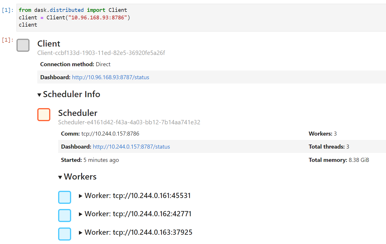
Walk through the examples to validate that the dask cluster is setup correctly, and that GPUs are accessible for the workers.
Worker metrics can be examined in dask dashboard.
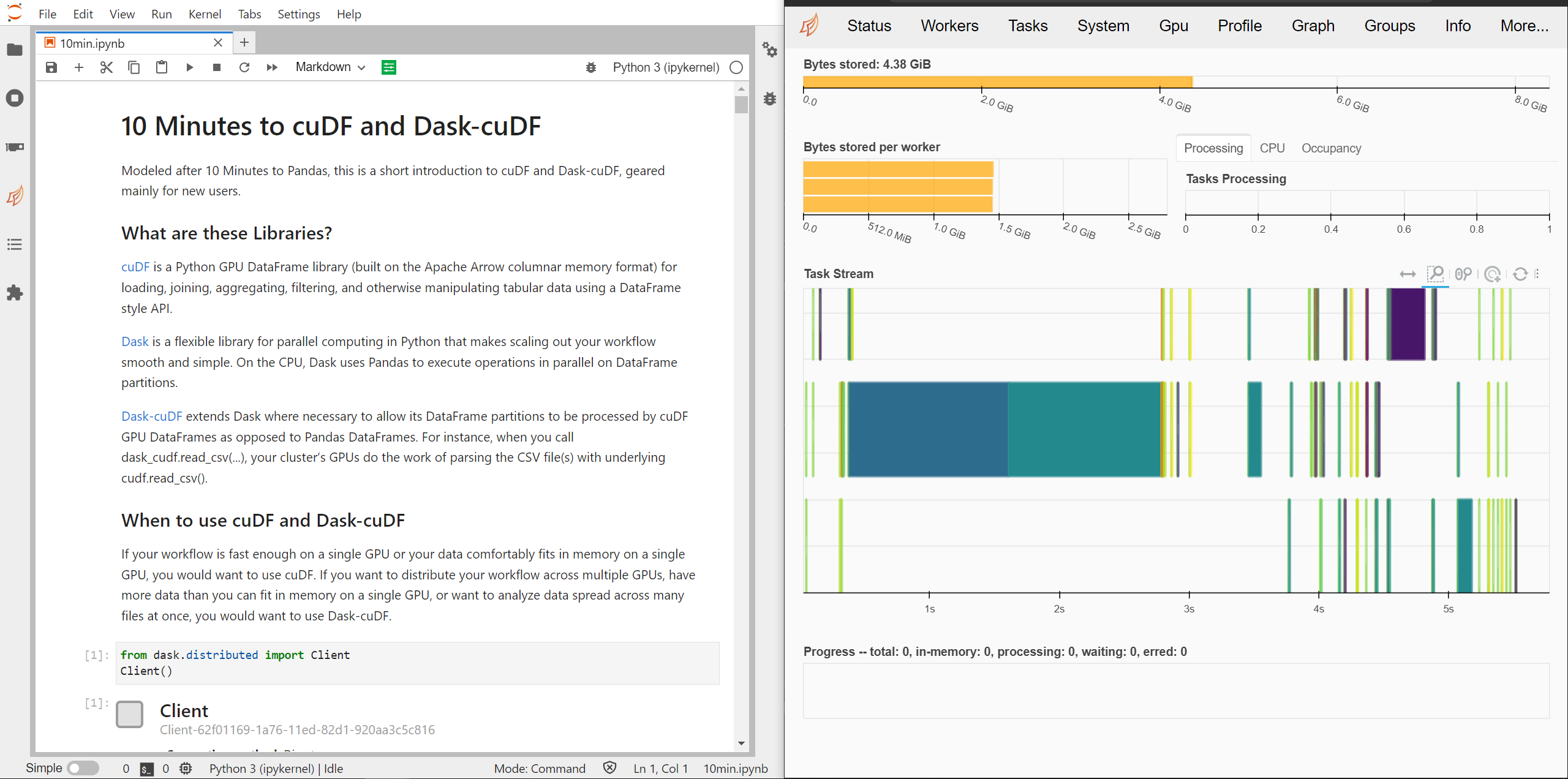
In case you want to scale up the cluster with more GPU workers, you may do so via `kubectl` or via `helm upgrade`.
```bash
$ kubectl scale deployment rapids-release-dask-worker --replicas=8
```
or
```bash
$ helm upgrade --set worker.replicas=8 rapids-release dask/dask
```
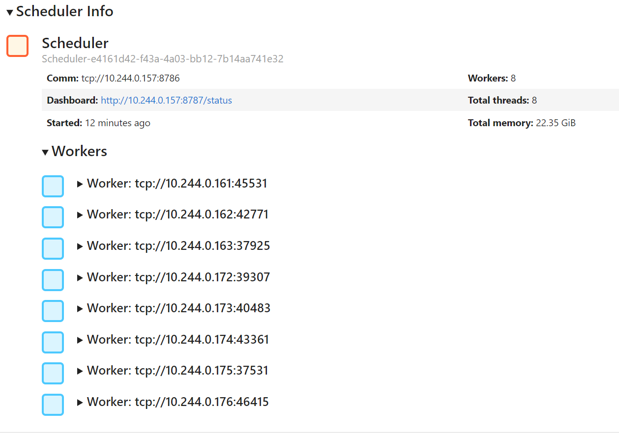
# index.html.md
# Measuring Performance with the One Billion Row Challenge
*January, 2024*
The [One Billion Row Challenge](https://www.morling.dev/blog/one-billion-row-challenge/) is a programming competition aimed at Java developers to write the most efficient code to process a one billion line text file and calculate some metrics. The challenge has inspired solutions in many languages beyond Java including [Python](https://github.com/gunnarmorling/1brc/discussions/62).
In this notebook we will explore how we can use RAPIDS to build an efficient solution in Python and how we can use dashboards to understand how performant our code is.
## The Problem
The input data of the challenge is a ~13GB text file containing one billion lines of temperature measurements. The file is structured with one measurement per line with the name of the weather station and the measurement separated by a semicolon.
```text
Hamburg;12.0
Bulawayo;8.9
Palembang;38.8
St. John's;15.2
Cracow;12.6
...
```
Our goal is to calculate the min, mean, and max temperature per weather station sorted alphabetically by station name as quickly as possible.
## Reference Implementation
A reference implementation written with popular PyData tools would likely be something along the lines of the following Pandas code (assuming you have enough RAM to fit the data into memory).
```python
import pandas as pd
df = pd.read_csv(
"measurements.txt",
sep=";",
header=None,
names=["station", "measure"],
engine='pyarrow'
)
df = df.groupby("station").agg(["min", "max", "mean"])
df.columns = df.columns.droplevel()
df = df.sort_values("station")
```
Here we use `pandas.read_csv()` to open the text file and specify the `;` separator and also set some column names. We also set the engine to `pyarrow` to give us some extra performance out of the box.
Then we group the measurements by their station name and calculate the min, max and mean. Finally we sort the grouped dataframe by the station name.
Running this on a workstation with a 12-core CPU completes the task in around **4 minutes**.
## Deploying RAPIDS
To run this notebook we will need a machine with one or more GPUs. There are many ways you can get this:
- Have a laptop, desktop or workstation with GPUs.
- Run a VM on the cloud using [AWS EC2](../../cloud/aws/ec2.md), [Google Compute Engine](../../cloud/gcp/compute-engine.md), [Azure VMs](../../cloud/azure/azure-vm.md), etc.
- Use a managed notebook service like [SageMaker](../../cloud/aws/sagemaker.md), [Vertex AI](../../cloud/gcp/vertex-ai.md), [Azure ML](../../cloud/azure/azureml.md) or [Databricks](../../platforms/databricks.md).
- Run a container in a [Kubernetes cluster with GPUs](../../platforms/kubernetes.md).
Once you have a GPU machine you will need to [install RAPIDS](https://docs.rapids.ai/install/). You can do this with [pip](https://docs.rapids.ai/install#pip), [conda](https://docs.rapids.ai/install#conda) or [docker](https://docs.rapids.ai/install#docker).
We are also going to use Jupyter Lab with the RAPIDS [nvdashboard extension](https://github.com/rapidsai/jupyterlab-nvdashboard) and the [Dask Lab Extension](https://github.com/dask/dask-labextension) so that we can understand what our machine is doing. If you are using the Docker container these will already be installed for you, otherwise you will need to install them yourself.
### Dashboards
Once you have Jupyter up and running with the extensions installed and this notebook downloaded you can open some performance dashboards so we can monitor our hardware as our code runs.
Let’s start with nvdashboard which has the GPU icon in the left toolbar.
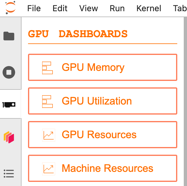
Start by opening the “Machine Resources” table, “GPU Utilization” graph and “GPU Memory” graph and moving them over to the right hand side.
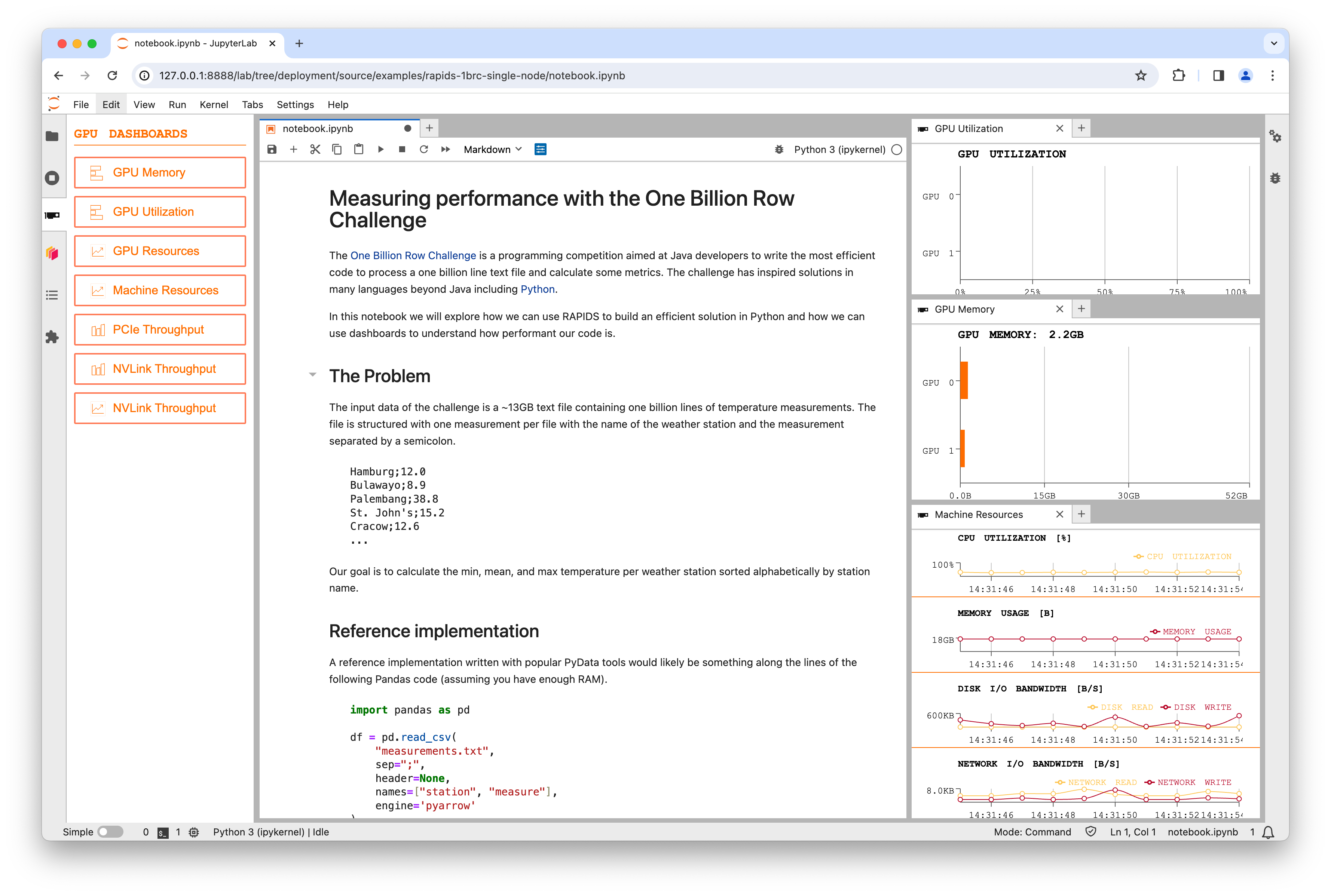
## Data Generation
Before we get started with our problem we need to generate the input data. The 1BRC repo has a [Java implementation](https://github.com/gunnarmorling/1brc/blob/main/src/main/java/dev/morling/onebrc/CreateMeasurements.java) which takes around 15 minutes to generate the file.
If you were to run the Java implementation you would see the CPU get busy but disk bandwidth remain low, suggesting this is a compute bound problem. We can accelerate this on the GPU using cuDF and CuPy.
Download the [`lookup.csv`](./lookup.csv) table of stations and their mean temperatures as we will use this to generate our data file containing `n` rows of random temperatures.
To generate each row we choose a random station from the lookup table, then generate a random temperature measurement from a normal distribution around the mean temp. We assume the standard deviation is `10.0` for all stations.
```ipython3
import time
from pathlib import Path
import cudf
import cupy as cp
```
```ipython3
def generate_chunk(filename, chunksize, std, lookup_df):
"""Generate some sample data based on the lookup table."""
df = cudf.DataFrame(
{
# Choose a random station from the lookup table for each row in our output
"station": cp.random.randint(0, len(lookup_df) - 1, int(chunksize)),
# Generate a normal distribution around zero for each row in our output
# Because the std is the same for every station we can adjust the mean for each row afterwards
"measure": cp.random.normal(0, std, int(chunksize)),
}
)
# Offset each measurement by the station's mean value
df.measure += df.station.map(lookup_df.mean_temp)
# Round the temperature to one decimal place
df.measure = df.measure.round(decimals=1)
# Convert the station index to the station name
df.station = df.station.map(lookup_df.station)
# Append this chunk to the output file
with open(filename, "a") as fh:
df.to_csv(fh, sep=";", chunksize=10_000_000, header=False, index=False)
```
### Configuration
```ipython3
n = 1_000_000_000 # Number of rows of data to generate
lookup_df = cudf.read_csv(
"lookup.csv"
) # Load our lookup table of stations and their mean temperatures
std = 10.0 # We assume temperatures are normally distributed with a standard deviation of 10
chunksize = 2e8 # Set the number of rows to generate in one go (reduce this if you run into GPU RAM limits)
filename = Path("measurements.txt") # Choose where to write to
filename.unlink() if filename.exists() else None # Delete the file if it exists already
```
### Run the data generation
```ipython3
%%time
# Loop over chunks and generate data
start = time.time()
for i in range(int(n / chunksize)):
# Generate a chunk
generate_chunk(filename, chunksize, std, lookup_df)
# Update the progress bar
percent_complete = int(((i + 1) * chunksize) / n * 100)
time_taken = int(time.time() - start)
time_remaining = int((time_taken / percent_complete) * 100) - time_taken
print(
(
f"Writing {int(n / 1e9)} billion rows to {filename}: {percent_complete}% "
f"in {time_taken}s ({time_remaining}s remaining)"
),
end="\r",
)
print()
```
```myst-ansi
Writing 1 billion rows to measurements.txt: 100% in 25s (0s remaining)
CPU times: user 10.1 s, sys: 18 s, total: 28.2 s
Wall time: 25.3 s
```
If you watch the graphs while this cell is running you should see a burts of GPU utilization when the GPU generates the random numbers followed by a burst of Disk IO when that data is written to disk. This pattern will happen for each chunk that is generated.
#### NOTE
We could improve performance even further here by generating the next chunk while the current chunk is writing to disk, but a 30x speedup seems optimal enough for now.
### Check the files
Now we can verify our dataset is the size we expected and contains rows that follow the format needed by the challenge.
```ipython3
!ls -lh {filename}
```
```myst-ansi
-rw-r--r-- 1 rapids conda 13G Jan 22 16:54 measurements.txt
```
```ipython3
!head {filename}
```
```myst-ansi
Guatemala City;17.3
Launceston;24.3
Bulawayo;8.7
Tbilisi;9.5
Napoli;26.8
Sarajevo;27.5
Chihuahua;29.2
Ho Chi Minh City;8.4
Johannesburg;19.2
Cape Town;16.3
```
## GPU Solution with RAPIDS
Now let’s look at using RAPIDS to speed up our Pandas implementation of the challenge. If you directly convert the reference implementation from Pandas to cuDF you will run into some [limitations cuDF has with string columns](https://github.com/rapidsai/cudf/issues/13733). Also depending on your GPU you may run into memory limits as cuDF will read the whole dataset into memory and machines typically have less GPU memory than CPU memory.
Therefore to solve this with RAPIDS we also need to use [Dask](https://dask.org) to partition the dataset and stream it through GPU memory, then cuDF can process each partition in a performant way.
### Deploying Dask
We are going to use [dask-cuda](../../tools/dask-cuda.md) to start a GPU Dask cluster.
```ipython3
from dask.distributed import Client
from dask_cuda import LocalCUDACluster
client = Client(LocalCUDACluster())
```
Creating a `LocalCUDACluster()` inspects the machine and starts one Dask worker for each detected GPU. We then pass that to a Dask client which means that all following code in the notebook will leverage the GPU workers.
### Dask Dashboard
We can also make use of the [Dask Dashboard](https://docs.dask.org/en/latest/dashboard.html) to see what is going on.
If you select the Dask logo from the left-hand toolbar and then click the search icon it should detect our `LocalCUDACluster` automatically and show us a long list of graphs to choose from.
When working with GPUs the “GPU Utilization” and “GPU Memory” will show us the same as the nvdashboard plots but for all machines in our Dask cluster. This is very helpful when working on a multi-node cluster but doesn’t help us in thie single-node configuration.
To see what Dask is doing in this challenge you should open the “Progress” and “Task Stream” graphs which will show all of the operations being performed. But feel free to open other graphs and explore all of the different metrics Dask can give you.
### Dask + cuDF Solution
Now that we have our input data and a Dask cluster we can write some Dask code that leverages cuDF under the hood to perform the compute operations.
First we need to import `dask.dataframe` and tell it to use the `cudf` backend.
```ipython3
import dask
import dask.dataframe as dd
dask.config.set({"dataframe.backend": "cudf"})
```
Now we can run our Dask code, which is almost identical to the Pandas code we used before.
```ipython3
%%timeit -n 3 -r 4
df = dd.read_csv("measurements.txt", sep=";", header=None, names=["station", "measure"])
df = df.groupby("station").agg(["min", "max", "mean"])
df.columns = df.columns.droplevel()
# We need to switch back to Pandas for the final sort at the time of writing due to rapidsai/cudf#14794
df = df.compute().to_pandas()
df = df.sort_values("station")
```
```myst-ansi
4.59 s ± 124 ms per loop (mean ± std. dev. of 4 runs, 3 loops each)
```
Running this notebook on a desktop workstation with two NVIDIA RTX 8000 GPUs completes the challenge in around **4 seconds** (a **60x speedup** over Pandas).
Watching the progress bars you should see them fill and reset a total of 12 times as our `%%timeit` operation is solving the challenge multiple times to get an average speed.
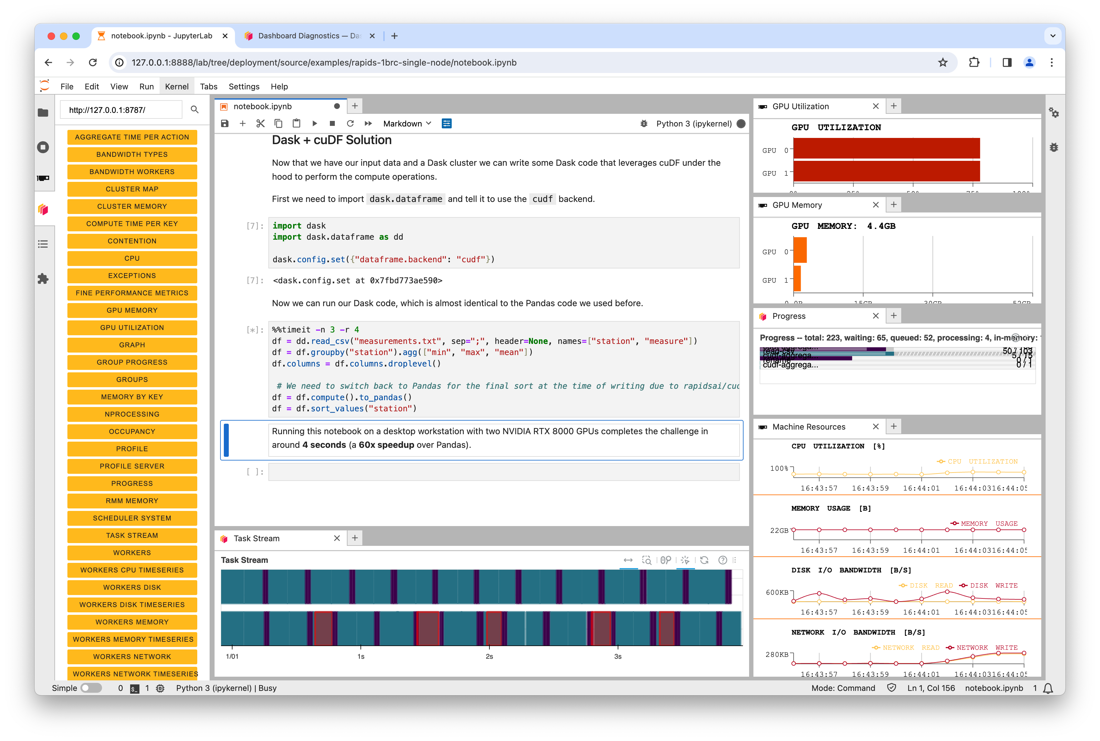
In the above screenshot you can see that on a dual-GPU system Dask was leveraging both GPUs. But it’s also interesting to note that the GPU utilization never reaches 100%. This is because the SSD in the machine has now become the bottleneck. The GPUs are performing the calculations so efficiently that we can’t read data from disk fast enough to fully saturate them.
# Conclusion
RAPIDS can accelerate existing workflows written with libraries like Pandas with little to no code changes. GPUs can accelerate computations by orders of magnitude which can move performance bottlenecks to other parts of the system.
Using dashboarding tools like nvdashboard and the Dask dashboard allow you to see and understand how your system is performing. Perhaps in this example upgrading the SSD is the next step to achieving even more performance.
# index.html.md
# HPO Benchmarking with RAPIDS and Dask
*August, 2023*
Hyper-Parameter Optimization (HPO) helps to find the best version of a model by exploring the space of possible configurations. While generally desirable, this search is computationally expensive and time-consuming.
In the notebook demo below, we compare benchmarking results to show how GPU can accelerate HPO tuning jobs relative to CPU.
For instance, we find a 48x speedup in wall clock time (0.71 hrs vs 34.6 hrs) for XGBoost and 16x (3.86 hrs vs 63.2 hrs) for RandomForest when comparing between `p3.8xlarge` Tesla V100 GPUs and `c5.24xlarge` CPU EC2 instances on 100 HPO trials of the 3-year Airline Dataset.
**Preamble**
You can set up local environment but it is recommended to launch a Virtual Machine service (Azure, AWS, GCP, etc).
For the purposes of this notebook, we will be utilizing the [Amazon Machine Image (AMI)](https://aws.amazon.com/releasenotes/aws-deep-learning-ami-gpu-tensorflow-2-12-amazon-linux-2/) as the starting point.
**Python ML Workflow**
In order to work with RAPIDS container, the entrypoint logic should parse arguments, load, preprocess and split data, build and train a model, score/evaluate the trained model, and emit an output representing the final score for the given hyperparameter setting.
Let’s have a step-by-step look at each stage of the ML workflow:
Dataset
We leverage the `Airline` dataset, which is a large public tracker of US domestic flight logs which we offer in various sizes (1 year, 3 year, and 10 year) and in [Parquet](https://parquet.apache.org/) (compressed column storage) format. The machine learning objective with this dataset is to predict whether flights will be more than 15 minutes late arriving to their destination.
We host the demo dataset in public S3 demo buckets in both the `us-east-1` or `us-west-2`. To optimize performance, we recommend that you access the s3 bucket in the same region as your EC2 instance to reduce network latency and data transfer costs.
For this demo, we are using the **`3_year`** dataset, which includes the following features to mention a few:
* Date and distance ( Year, Month, Distance )
* Airline / carrier ( Flight_Number_Reporting_Airline )
* Actual departure and arrival times ( DepTime and ArrTime )
* Difference between scheduled & actual times ( ArrDelay and DepDelay )
* Binary encoded version of late, aka our target variable ( ArrDelay15 )
Configure aws credentials for access to S3 storage
```default
aws configure
```
Download dataset from S3 bucket to your current working dir
```default
aws s3 cp --recursive s3://sagemaker-rapids-hpo-us-west-2/3_year/ ./data/
```
Algorithm
From a ML/algorithm perspective, we offer `XGBoost` and `RandomForest`. You are free to switch between these algorithm choices and everything in the example will continue to work.
```python
parser = argparse.ArgumentParser()
parser.add_argument(
"--model-type", type=str, required=True, choices=["XGBoost", "RandomForest"]
)
```
We can also optionally increase robustness via reshuffles of the train-test split (i.e., cross-validation folds). Typical values are between 3 and 10 folds. We will use
```python
n_cv_folds = 5
```
Dask Cluster
To maximize on efficiency, we launch a Dask `LocalCluster` for cpu or `LocalCUDACluster` that utilizes GPUs for distributed computing. Then connect a Dask Client to submit and manage computations on the cluster.
We can then ingest the data, and “persist” it in memory using dask as follows:
```python
if args.mode == "gpu":
cluster = LocalCUDACluster()
else: # mode == "cpu"
cluster = LocalCluster(n_workers=os.cpu_count())
with Client(cluster) as client:
dataset = ingest_data(mode=args.mode)
client.persist(dataset)
```
Search Range
One of the most important choices when running HPO is to choose the bounds of the hyperparameter search process. In this notebook, we leverage the power of `Optuna`, a widely used Python library for hyperparameter optimization.
Here’s the quick steps on getting started with Optuna:
1. Define the Objective Function, which represents the model training and evaluation process. It takes hyperparameters as inputs and returns a metric to optimize (e.g, accuracy in our case,). Refer to `train_xgboost()` and `train_randomforest()` in `hpo.py`
1. Specify the search space using the `Trial` object’s methods to define the hyperparameters and their corresponding value ranges or distributions. For example:
```python
"max_depth": trial.suggest_int("max_depth", 4, 8),
"max_features": trial.suggest_float("max_features", 0.1, 1.0),
"learning_rate": trial.suggest_float("learning_rate", 0.001, 0.1, log=True),
"min_samples_split": trial.suggest_int("min_samples_split", 2, 1000, log=True),
```
1. Create an Optuna study object to keep track of trials and their corresponding hyperparameter configurations and evaluation metrics.
```python
study = optuna.create_study(
sampler=RandomSampler(seed=args.seed), direction="maximize"
)
```
1. Select an optimization algorithm to determine how Optuna explores and exploits the search space to find optimal configurations. For instance, the `RandomSampler` is an algorithm provided by the Optuna library that samples hyperparameter configurations randomly from the search space.
2. Run the Optimization by calling the Optuna’s `optimize()` function on the study object. You can specify the number of trials or number of parallel jobs to run.
```python
study.optimize(lambda trial: train_xgboost(
trial, dataset=dataset, client=client, mode=args.mode
),
n_trials=100,
n_jobs=1,
)
```
**Run HPO**
Let’s try this out!
The example file `hpo.py` included here implements the patterns described above.
First make sure you have the correct CUDAtoolkit version by running `nvidia-smi`. See the RAPIDS installation docs ([link](https://docs.rapids.ai/install/#system-req)) for details on the supported range of GPUs and drivers.
```ipython3
!nvidia-smi
```
Executing benchmark tests can be an arduous and time-consuming procedure that may extend over multiple days. By using a tool like [tmux](https://www.redhat.com/sysadmin/introduction-tmux-linux), you can maintain active terminal sessions, ensuring that your tasks continue running even if the SSH connection is interrupted.
```default
tmux
```
Run the following to run hyper-parameter optimization in a Docker container.
If you don’t yet have that image locally, the first time this runs it might take a few minutes to pull it.
After that, startup should be very fast.
Here’s what the arguments in that command below are doing:
* `--gpus all` = make all GPUs on the system available to processes in the container
* `--env EXTRA_CONDA_PACKAGES` = install `optuna` and `optuna-integration` conda packages
- *the image already comes with all of the RAPIDS libraries and their dependencies installed*
* `-p 8787:8787` = forward between port port 8787 on the host and 8787 on the container
- *navigate to \`{public IP of box}:8787 to see the Dask dashboard!*
* `-v / -w` = mount the current directory from the host machine into the container
- *this allows processes in the container to read the data you downloaded to the `./data` directory earlier*
- *it also means that any changes made to these files from inside the container will be reflected back on the host*
Piping to a file called `xgboost_hpo_logs.txt` is helpful, as it preserves all the logs for later inspection.
```ipython3
!docker run \
--gpus all \
--env EXTRA_CONDA_PACKAGES="optuna optuna-integration" \
-p 8787:8787 \
-v $(pwd):/home/rapids/xgboost-hpo-example \
-w /home/rapids/xgboost-hpo-example \
-it rapidsai/base:25.12a-cuda12-py3.13 \
/bin/bash -c "python ./hpo.py --model-type 'XGBoost' --target 'gpu'" \
> ./xgboost_hpo_logs.txt 2>&1
```
**Try Some Modifications**
Now that you’ve run this example, try some modifications!
For example:
* use `--model-type "RandomForest"` to see how a random forest model compares to XGBoost
* use `--target "cpu"` to estimate the speedup from GPU-accelerated training
* modify the pipeline in `hpo.py` with other customizations
# index.html.md
# Scaling up Hyperparameter Optimization with Kubernetes and XGBoost GPU Algorithm
*January, 2023*
Choosing an optimal set of hyperparameters is a daunting task, especially for algorithms like XGBoost that have many hyperparameters to tune. In this notebook, we will show how to speed up hyperparameter optimization by running multiple training jobs in parallel on a Kubernetes cluster.
# Prerequisites
Please follow instructions in [Dask Operator: Installation](../../tools/kubernetes/dask-operator.md) to install the Dask operator on top of a GPU-enabled Kubernetes cluster. (For the purpose of this example, you may ignore other sections of the linked document.)
## Optional: Kubeflow
Kubeflow gives you a nice notebook environment to run this notebook within the k8s cluster. Install Kubeflow by following instructions in [Installing Kubeflow](https://www.kubeflow.org/docs/started/installing-kubeflow/). You may choose any method; we tested this example after installing Kubeflow from manifests.
# Install system packages
We’ll need extra Python packages. In particular, we need an unreleased version of Optuna:
```ipython3
!pip install dask_kubernetes optuna optuna-integration
```
# Set up Dask cluster
Let us set up a Dask cluster using the `KubeCluster` class. Fill in the following variables, depending on the configuration of your Kubernetes cluster. Here how you can get `n_workers`, assuming that you are using all the nodes in the Kubernetes cluster. Let `N` be the number of nodes.
* On AWS Elastic Kubernetes Service (EKS): `n_workers = N - 2`
* On Google Cloud Kubernetes: `n_workers = N - 1`
```ipython3
# Choose the same RAPIDS image you used for launching the notebook session
rapids_image = "rapidsai/base:25.12a-cuda12-py3.13"
# Use the number of worker nodes in your Kubernetes cluster.
n_workers = 4
```
```ipython3
from dask_kubernetes.operator import KubeCluster
cluster = KubeCluster(
name="rapids-dask",
image=rapids_image,
worker_command="dask-cuda-worker",
n_workers=n_workers,
resources={"limits": {"nvidia.com/gpu": "1"}},
env={"EXTRA_PIP_PACKAGES": "optuna"},
)
```
```myst-ansi
Unclosed client session
client_session:
```
```ipython3
cluster
```
```ipython3
from dask.distributed import Client
client = Client(cluster)
```
# Perform hyperparameter optimization with a toy example
Now we can run hyperparameter optimization. The workers will run multiple training jobs in parallel.
```ipython3
def objective(trial):
x = trial.suggest_uniform("x", -10, 10)
return (x - 2) ** 2
```
```ipython3
import optuna
from dask.distributed import wait
# Number of hyperparameter combinations to try in parallel
n_trials = 100
# Optimize in parallel on your Dask cluster
backend_storage = optuna.storages.InMemoryStorage()
dask_storage = optuna.integration.DaskStorage(storage=backend_storage, client=client)
study = optuna.create_study(direction="minimize", storage=dask_storage)
futures = []
for i in range(0, n_trials, n_workers * 4):
iter_range = (i, min([i + n_workers * 4, n_trials]))
futures.append(
{
"range": iter_range,
"futures": [
client.submit(study.optimize, objective, n_trials=1, pure=False)
for _ in range(*iter_range)
],
}
)
for partition in futures:
iter_range = partition["range"]
print(f"Testing hyperparameter combinations {iter_range[0]}..{iter_range[1]}")
_ = wait(partition["futures"])
```
```myst-ansi
/tmp/ipykernel_75/1194069379.py:9: ExperimentalWarning: DaskStorage is experimental (supported from v3.1.0). The interface can change in the future.
dask_storage = optuna.integration.DaskStorage(storage=backend_storage, client=client)
```
```myst-ansi
Testing hyperparameter combinations 0..16
Testing hyperparameter combinations 16..32
Testing hyperparameter combinations 32..48
Testing hyperparameter combinations 48..64
Testing hyperparameter combinations 64..80
Testing hyperparameter combinations 80..96
Testing hyperparameter combinations 96..100
```
```ipython3
study.best_params
```
```ipython3
study.best_value
```
# Perform hyperparameter optimization with XGBoost GPU algorithm
Now let’s try optimizing hyperparameters for an XGBoost model.
```ipython3
import xgboost as xgb
from optuna.samplers import RandomSampler
from sklearn.datasets import load_breast_cancer
from sklearn.model_selection import KFold, cross_val_score
def objective(trial):
X, y = load_breast_cancer(return_X_y=True)
params = {
"n_estimators": 10,
"verbosity": 0,
"tree_method": "gpu_hist",
# L2 regularization weight.
"lambda": trial.suggest_float("lambda", 1e-8, 100.0, log=True),
# L1 regularization weight.
"alpha": trial.suggest_float("alpha", 1e-8, 100.0, log=True),
# sampling according to each tree.
"colsample_bytree": trial.suggest_float("colsample_bytree", 0.2, 1.0),
"max_depth": trial.suggest_int("max_depth", 2, 10, step=1),
# minimum child weight, larger the term more conservative the tree.
"min_child_weight": trial.suggest_float(
"min_child_weight", 1e-8, 100, log=True
),
"learning_rate": trial.suggest_float("learning_rate", 1e-8, 1.0, log=True),
# defines how selective algorithm is.
"gamma": trial.suggest_float("gamma", 1e-8, 1.0, log=True),
"grow_policy": "depthwise",
"eval_metric": "logloss",
}
clf = xgb.XGBClassifier(**params)
fold = KFold(n_splits=5, shuffle=True, random_state=0)
score = cross_val_score(clf, X, y, cv=fold, scoring="neg_log_loss")
return score.mean()
```
```ipython3
# Number of hyperparameter combinations to try in parallel
n_trials = 250
# Optimize in parallel on your Dask cluster
backend_storage = optuna.storages.InMemoryStorage()
dask_storage = optuna.integration.DaskStorage(storage=backend_storage, client=client)
study = optuna.create_study(
direction="maximize", sampler=RandomSampler(seed=0), storage=dask_storage
)
futures = []
for i in range(0, n_trials, n_workers * 4):
iter_range = (i, min([i + n_workers * 4, n_trials]))
futures.append(
{
"range": iter_range,
"futures": [
client.submit(study.optimize, objective, n_trials=1, pure=False)
for _ in range(*iter_range)
],
}
)
for partition in futures:
iter_range = partition["range"]
print(f"Testing hyperparameter combinations {iter_range[0]}..{iter_range[1]}")
_ = wait(partition["futures"])
```
```myst-ansi
/tmp/ipykernel_75/1634478960.py:6: ExperimentalWarning: DaskStorage is experimental (supported from v3.1.0). The interface can change in the future.
dask_storage = optuna.integration.DaskStorage(storage=backend_storage, client=client)
```
```myst-ansi
Testing hyperparameter combinations 0..16
Testing hyperparameter combinations 16..32
Testing hyperparameter combinations 32..48
Testing hyperparameter combinations 48..64
Testing hyperparameter combinations 64..80
Testing hyperparameter combinations 80..96
Testing hyperparameter combinations 96..112
Testing hyperparameter combinations 112..128
Testing hyperparameter combinations 128..144
Testing hyperparameter combinations 144..160
Testing hyperparameter combinations 160..176
Testing hyperparameter combinations 176..192
Testing hyperparameter combinations 192..208
Testing hyperparameter combinations 208..224
Testing hyperparameter combinations 224..240
Testing hyperparameter combinations 240..250
```
```ipython3
study.best_params
```
```ipython3
study.best_value
```
Let’s visualize the progress made by hyperparameter optimization.
```ipython3
from optuna.visualization.matplotlib import (
plot_optimization_history,
plot_param_importances,
)
```
```ipython3
plot_optimization_history(study)
```
```myst-ansi
/tmp/ipykernel_75/3324289224.py:1: ExperimentalWarning: plot_optimization_history is experimental (supported from v2.2.0). The interface can change in the future.
plot_optimization_history(study)
```
```ipython3
plot_param_importances(study)
```
```myst-ansi
/tmp/ipykernel_75/3836449081.py:1: ExperimentalWarning: plot_param_importances is experimental (supported from v2.2.0). The interface can change in the future.
plot_param_importances(study)
```
# index.html.md
# Getting Started with cuML’s accelerator mode (cuml.accel) in Snowflake Notebooks
*July, 2025*
cuML is a Python GPU library for accelerating machine learning models using a scikit-learn-like API.
cuML now has an accelerator mode (cuml.accel) which allows you to bring accelerated computing to existing workflows with zero code changes required. In addition to scikit-learn, cuml.accel also provides acceleration to algorithms found in umap-learn (UMAP) and hdbscan (HDBSCAN).
This notebook is a brief introduction to cuml.accel.
# ⚠️ Verify your setup
First, we’ll verify that we are running on an NVIDIA GPU:
```ipython3
!nvidia-smi # this should display information about available GPUs
```
With classical machine learning, there is a wide range of interesting problems we can explore. In this tutorial we’ll examine 3 of the more popular use cases: classification, clustering, and dimensionality reduction.
# Classification
Let’s load a dataset and see how we can use scikit-learn to classify that data. For this example we’ll use the Coverage Type dataset, which contains a number of features that can be used to predict forest cover type, such as elevation, aspect, slope, and soil-type.
More information on this dataset can be found at https://archive.ics.uci.edu/dataset/31/covertype.
```ipython3
import pandas as pd
from sklearn.ensemble import RandomForestClassifier
from sklearn.metrics import accuracy_score, classification_report
from sklearn.model_selection import train_test_split
```
```ipython3
url = (
"https://archive.ics.uci.edu/ml/machine-learning-databases/covtype/covtype.data.gz"
)
# Column names for the dataset (from UCI Covertype description)
columns = [
"Elevation",
"Aspect",
"Slope",
"Horizontal_Distance_To_Hydrology",
"Vertical_Distance_To_Hydrology",
"Horizontal_Distance_To_Roadways",
"Hillshade_9am",
"Hillshade_Noon",
"Hillshade_3pm",
"Horizontal_Distance_To_Fire_Points",
"Wilderness_Area1",
"Wilderness_Area2",
"Wilderness_Area3",
"Wilderness_Area4",
"Soil_Type1",
"Soil_Type2",
"Soil_Type3",
"Soil_Type4",
"Soil_Type5",
"Soil_Type6",
"Soil_Type7",
"Soil_Type8",
"Soil_Type9",
"Soil_Type10",
"Soil_Type11",
"Soil_Type12",
"Soil_Type13",
"Soil_Type14",
"Soil_Type15",
"Soil_Type16",
"Soil_Type17",
"Soil_Type18",
"Soil_Type19",
"Soil_Type20",
"Soil_Type21",
"Soil_Type22",
"Soil_Type23",
"Soil_Type24",
"Soil_Type25",
"Soil_Type26",
"Soil_Type27",
"Soil_Type28",
"Soil_Type29",
"Soil_Type30",
"Soil_Type31",
"Soil_Type32",
"Soil_Type33",
"Soil_Type34",
"Soil_Type35",
"Soil_Type36",
"Soil_Type37",
"Soil_Type38",
"Soil_Type39",
"Soil_Type40",
"Cover_Type",
]
data = pd.read_csv(url, header=None)
data.columns = columns
```
```ipython3
data.shape
```
Next, we’ll separate out the classification variable (Cover_Type) from the rest of the data. This is what we will aim to predict with our classification model. We can also split our dataset into training and test data using the scikit-learn train_test_split function.
```ipython3
X, y = data.drop("Cover_Type", axis=1), data["Cover_Type"]
X_train, X_test, y_train, y_test = train_test_split(X, y, test_size=0.2)
```
Now that we have our dataset split, we’re ready to run a model. To start, we will just run the model using the sklearn library with a starting max depth of 5 and all of the features. Note that we can set n_jobs=-1 to utilize all available CPU cores for fitting the trees – this will ensure we get the best performance possible on our system’s CPU.
```ipython3
import time
```
```ipython3
# Start timing cpu
start_time_cpu = time.time()
clf = RandomForestClassifier(n_estimators=100, max_depth=5, max_features=1.0, n_jobs=-1)
clf.fit(X_train, y_train)
# End timing
end_time_cpu = time.time()
```
```ipython3
# Report CPU duration
print(f"CPU Training completed in {end_time_cpu - start_time_cpu:.2f} seconds")
```
In about 38 seconds, we were able to fit our tree model using scikit-learn. This is not bad! Let’s use the model we just trained to predict coverage types in our test dataset and take a look at the accuracy of our model.
```ipython3
y_pred = clf.predict(X_test)
accuracy_score(y_test, y_pred)
```
We can also print out a full classification report to better understand how we predicted different Coverage_Type categories.
```ipython3
print(classification_report(y_test, y_pred))
```
With scikit-learn, we built a model that was able to be trained in just less than a minute. From the accuracy report, we can see that we predicted the correct class around 70% of the time, which is not bad but could certainly be improved.
Now let’s load cuml.accel and try running the same code again to see what kind of acceleration we can get.
```ipython3
import cuml.accel
cuml.accel.install()
```
**IMPORTANT:** After installing cuml.accel, we need to import the scikit-learn estimators we wish to use again.
```ipython3
from sklearn.ensemble import RandomForestClassifier
```
```ipython3
# Start timing gpu
start_time_gpu = time.time()
clf = RandomForestClassifier(n_estimators=100, max_depth=5, max_features=1.0, n_jobs=-1)
clf.fit(X_train, y_train)
# End timing
end_time_gpu = time.time()
```
```ipython3
# Report GPU duration
print(f"GPU Training completed in {end_time_gpu - start_time_gpu:.2f} seconds")
```
That was much faster! Using cuML we’re able to train this random forest model in just 3.5 seconds, that’s more than 10X speedup. One thing to note is that cuML’s implementation of `RandomForestClassifier` doesn’t utilize the `n_jobs` parameter like scikit-learn, but we still accept it which makes it easier to use this accelerator with zero code changes.
Let’s take a look at the same accuracy score and classification report to compare the model’s performance.
```ipython3
y_pred = clf.predict(X_test)
cr = classification_report(y_test, y_pred)
print(cr)
```
Out of the box, the model performed about the same as the scikit-learn implementation. Because this model ran so much faster, we can quickly iterate on the hyperparameter configuration and find a model that performs better with excellent speedups.
```ipython3
# Start timing gpu max_depth 30
start_time_gpu_md30 = time.time()
clf = RandomForestClassifier(
n_estimators=100, max_depth=30, max_features=1.0, n_jobs=-1
)
clf.fit(X_train, y_train)
# End timing
end_time_gpu_md30 = time.time()
# Report GPU duration
print(
f"GPU Training with max_depth=30 completed in {end_time_gpu_md30 - start_time_gpu_md30:.2f} seconds"
)
```
```ipython3
y_pred = clf.predict(X_test)
print(classification_report(y_test, y_pred))
```
We just run a model in a few seconds, and got a better accuracy. With a model that runs in just seconds, we can perform hyperparameter optimization using a method like the grid search shown above, and have results in just minutes instead of hours.
## Resources
For more information on getting started with `cuml.accel`, check out [RAPIDS.ai](https://rapids.ai/cuml-accel/) or the [cuML Docs](https://docs.rapids.ai/api/cuml/stable/).
Find more examples of usage in this [cuml_sklearn_demo](https://colab.research.google.com/github/rapidsai-community/showcase/blob/main/getting_started_tutorials/cuml_sklearn_colab_demo.ipynb)
# index.html.md
# Getting Started with Optuna and RAPIDS for HPO
*March, 2023*
Hyperparameter optimization (HPO) automates the process of picking values for the hyperparameters of a machine learning algorithm to improve model performance. This can help boost the model accuracy, but can be resource-intensive, as it may require training the model for hundreds of hyperparameter combinations. Let’s take a look at how we can use Optuna and RAPIDS to make HPO less time-consuming.
## RAPIDS
The RAPIDS framework provides a suite of libraries to execute end-to-end data science pipelines entirely on GPUs. One of the libraries in this framework is cuML, which implements common machine learning models with a scikit-learn-compatible API and a GPU-accelerated backend. You can learn more about RAPIDS [here](https://rapids.ai/about.html).
## Optuna
[Optuna](https://optuna.readthedocs.io/en/stable/) is a lightweight framework for automatic hyperparameter optimization. It provides a define-by-run API, which makes it easy to adapt to any already existing code that we have and enables high modularity along with the flexibility to construct hyperparameter spaces dynamically. By simply wrapping the objective function with Optuna, we can perform a parallel-distributed HPO search over a search space as we’ll see in this notebook.
In this notebook, we’ll use BNP Paribas Cardif Claims Management dataset from Kaggle to predict if a claim will receive accelerated approval or not. We’ll explore how to use Optuna with RAPIDS in combination with Dask to run multi-GPU HPO experiments that can yield results faster than CPU.
```ipython3
## Run this cell to install optuna
#!pip install optuna optuna-integration
```
```ipython3
import cudf
import optuna
from cuml import LogisticRegression
from cuml.metrics import log_loss
from cuml.model_selection import train_test_split
from dask.distributed import Client, wait
from dask_cuda import LocalCUDACluster
```
## Set up CUDA Cluster
We start a local cluster and keep it ready for running distributed tasks with dask. The dask scheduler can help leverage multiple nodes available on the cluster.
[LocalCUDACluster](https://github.com/rapidsai/dask-cuda) launches one Dask worker for each GPU in the current systems. It’s developed as a part of the RAPIDS project. Learn More:
- [Setting up Dask](https://docs.dask.org/en/latest/setup.html)
- [Dask Client](https://distributed.dask.org/en/latest/client.html)
```ipython3
# This will use all GPUs on the local host by default
cluster = LocalCUDACluster(threads_per_worker=1, ip="", dashboard_address="8081")
c = Client(cluster)
# Query the client for all connected workers
workers = c.has_what().keys()
n_workers = len(workers)
c
```
```myst-ansi
[I 2024-08-06 09:41:38,254] A new study created in memory with name: dask_optuna_lr_log_loss_tpe
```
# Loading the Data
## Data Acquisition
Dataset can be acquired from Kaggle: [BNP Paribas Cardif Claims Management](https://www.kaggle.com/c/bnp-paribas-cardif-claims-management/data). To download the dataset:
1. Follow the instructions here to: [Set-up the Kaggle API](https://github.com/Kaggle/kaggle-api)
2. Run the following to download the data
```shell
mkdir -p ./data
kaggle competitions download \
-c bnp-paribas-cardif-claims-management \
--path ./data
unzip \
-d ./data \
./data/bnp-paribas-cardif-claims-management.zip
```
This is an anonymized dataset containing categorical and numerical values for claims received by BNP Paribas Cardif. The “target” column in the train set is the variable to predict. It is equal to 1 for claims suitable for an accelerated approval. The task is to predict whether a claim will be suitable for accelerated approval or not. We’ll only use the `train.csv.zip` file as `test.csv.zip` does not have a target column.
```ipython3
import os
file_name = "train.csv.zip"
data_dir = "data/"
INPUT_FILE = os.path.join(data_dir, file_name)
```
Select the `N_TRIALS` for the number of runs of HPO trials.
```ipython3
N_TRIALS = 150
df = cudf.read_csv(INPUT_FILE)
# Drop ID column
df = df.drop("ID", axis=1)
# Drop non-numerical data and fill NaNs before passing to cuML RF
CAT_COLS = list(df.select_dtypes("object").columns)
df = df.drop(CAT_COLS, axis=1)
df = df.fillna(0)
df = df.astype("float32")
X, y = df.drop(["target"], axis=1), df["target"].astype("int32")
study_name = "dask_optuna_lr_log_loss_tpe"
```
# Training and Evaluation
The `train_and_eval` function accepts the different parameters to try out. This function should look very similar to any ML workflow. We’ll use this function within the Optuna `objective` function to show how easily we can fit an existing workflow into the Optuna work.
```ipython3
def train_and_eval(
X_param, y_param, penalty="l2", C=1.0, l1_ratio=None, fit_intercept=True
):
"""
Splits the given data into train and test split to train and evaluate the model
for the params parameters.
Params
______
X_param: DataFrame.
The data to use for training and testing.
y_param: Series.
The label for training
penalty, C, l1_ratio, fit_intercept: The parameter values for Logistic Regression.
Returns
score: log loss of the fitted model
"""
X_train, X_valid, y_train, y_valid = train_test_split(
X_param, y_param, random_state=42
)
classifier = LogisticRegression(
penalty=penalty,
C=C,
l1_ratio=l1_ratio,
fit_intercept=fit_intercept,
max_iter=10000,
)
classifier.fit(X_train, y_train)
y_pred = classifier.predict(X_valid)
score = log_loss(y_valid, y_pred)
return score
```
For a baseline number, let’s see what the default performance of the model is.
```ipython3
print("Score with default parameters : ", train_and_eval(X, y))
```
```myst-ansi
[W] [09:34:11.132560] L-BFGS line search failed (code 3); stopping at the last valid step
Score with default parameters : 8.24908383066997
```
## Objective Function
We will optimize the objective function using [Optuna Study](https://optuna.readthedocs.io/en/stable/reference/study.html). The objective function tries out specified values for the parameters that we are tuning and returns the score obtained with those parameters. These results will be aggregated in `study.trials_dataframes()`.
Let’s define the objective function for this HPO task by making use of the `train_and_eval()`. You can see that we simply choose a value for the parameters and call the `train_and_eval` method, making Optuna very easy to use in an existing workflow.
The objective function does not need to be changed when switching to different [samplers](https://optuna.readthedocs.io/en/stable/reference/samplers.html), which are built-in options in Optuna to enable the selection of different sampling algorithms that optuna provides. Some of the available ones include - GridSampler, RandomSampler, TPESampler, etc. We’ll use TPESampler for this demo, but feel free to try different samplers to notice the changes in performance.
[Tree-Structured Parzen Estimators](https://optuna.readthedocs.io/en/stable/reference/generated/optuna.samplers.TPESampler.html#optuna.samplers.TPESampler) or TPE works by fitting two Gaussian Mixture Model during each trial - one to the set of parameter values associated with the best objective values,
and another to the remaining parameter values. It chooses the parameter value that maximizes the ratio between the two GMMs
```ipython3
def objective(trial, X_param, y_param):
C = trial.suggest_float("C", 0.01, 100.0, log=True)
penalty = trial.suggest_categorical("penalty", ["none", "l1", "l2"])
fit_intercept = trial.suggest_categorical("fit_intercept", [True, False])
score = train_and_eval(
X_param, y_param, penalty=penalty, C=C, fit_intercept=fit_intercept
)
return score
```
## HPO Trials and Study
Optuna uses [studies](https://optuna.readthedocs.io/en/stable/reference/study.html) and [trials](https://optuna.readthedocs.io/en/stable/reference/trial.html) to keep track of the HPO experiments. Put simply, a trial is a single call of the objective function while a set of trials make up a study. We will pick the best observed trial from a study to get the best parameters that were used in that run.
Here, `DaskStorage` class is used to set up a storage shared by all workers in the cluster. Learn more about what storages can be used [here](https://optuna.readthedocs.io/en/stable/reference/storages.html)
`optuna.create_study` is used to set up the study. As you can see, it specifies the study name, sampler to be used, the direction of the study, and the storage.
With just a few lines of code, we have set up a distributed HPO experiment.
```ipython3
storage = optuna.integration.DaskStorage()
study = optuna.create_study(
sampler=optuna.samplers.TPESampler(seed=142),
study_name=study_name,
direction="minimize",
storage=storage,
)
# Optimize in parallel on your Dask cluster
#
# Submit `n_workers` optimization tasks, where each task runs about 40 optimization trials
# for a total of about N_TRIALS trials in all
futures = [
c.submit(
study.optimize,
lambda trial: objective(trial, X, y),
n_trials=N_TRIALS // n_workers,
pure=False,
)
for _ in range(n_workers)
]
wait(futures)
print(f"Best params: {study.best_params}")
print("Number of finished trials: ", len(study.trials))
```
You should see logs like the following.
```text
[I 2024-08-06 09:41:40,161] Trial 1 finished with value: 8.238207899472073 and parameters: {'C': 40.573838784392514, 'penalty': 'l2', 'fit_intercept': True}. Best is trial 1 with value: 8.238207899472073.
...
[I 2024-08-06 09:41:58,423] Trial 143 finished with value: 8.210414278942531 and parameters: {'C': 0.3152731188939818, 'penalty': 'l1', 'fit_intercept': True}. Best is trial 52 with value: 8.205579602300705.
Best params: {'C': 1.486491072441749, 'penalty': 'l2', 'fit_intercept': True}
Number of finished trials: 144
```
## Visualization
Optuna provides an easy way to visualize the trials via builtin graphs. Read more about visualizations [here](https://optuna.readthedocs.io/en/stable/tutorial/10_key_features/005_visualization.html).
## Concluding Remarks
This notebook shows how RAPIDS and Optuna can be used along with dask to run multi-GPU HPO jobs, and can be used as a starting point for anyone wanting to get started with the framework. We have seen how by just adding a few lines of code we were able to integrate the libraries for a muli-GPU HPO runs. This can also be scaled to multiple nodes.
## Next Steps
This is done on a small dataset, you are encouraged to test out on larger data with more range for the parameters too. These experiments can yield performance improvements. Refer to other examples in the [rapidsai/cloud-ml-examples](https://github.com/rapidsai/cloud-ml-examples) repository.
## Resources
[Hyperparameter Tuning in Python](https://towardsdatascience.com/hyperparameter-tuning-c5619e7e6624)
[Overview of Hyperparameter tuning](https://cloud.google.com/ai-platform/training/docs/hyperparameter-tuning-overview)
[How to make your model awesome with Optuna](https://towardsdatascience.com/how-to-make-your-model-awesome-with-optuna-b56d490368af)
# index.html.md
# Training XGBoost with Dask RAPIDS in Databricks
*January, 2024*
This notebook shows how to deploy Dask RAPIDS workflow in Databricks. We will focus on the HIGGS dataset, a moderately sized classification problem from the [UCI Machine Learning repository.](https://archive.ics.uci.edu/dataset/280/higgs)
In the following sections, we will begin by loading the dataset from [Delta Lake](https://delta.io/) and performing preprocessing with [Dask](https://github.com/dask/dask). Then train an [XGBoost](https://xgboost.readthedocs.io/en/stable/) model with various configurations and explore techniques for optimizing inference.
## Launch multi-node Dask Cluster
This workflow example can be ran on GPU, and you don’t even need to have the GPU locally since Databricks can provide one for you. Whereas Dask enables users to easily distribute or scale up computation tasks within a single GPU or across multiple GPUs.
Dask recently introduced [**dask-databricks**](https://github.com/dask-contrib/dask-databricks) (available via [conda](https://github.com/conda-forge/dask-databricks-feedstock) and [pip](https://pypi.org/project/dask-databricks/)). With this CLI tool, the `dask databricks run --cuda` command will launch a Dask scheduler in the driver node and [`cuda` workers](https://docs.rapids.ai/api/dask-cuda/nightly) in the remaining nodes.
From a high level, we could break down this section into the following steps:
* Create a new [init script](https://docs.databricks.com/en/init-scripts/index.html) that installs [RAPIDS](https://rapids.ai/) and runs `dask-databricks`
* Create a new multi-node cluster that uses the init script
* Once the cluster is running upload this notebook to Databricks and continue running these cells on there
## Import packages
Once your cluster has launched, start by importing all necessary libraries and dependencies.
```ipython3
import os
import dask_cudf
import dask_databricks
import dask_deltatable as ddt
import numpy as np
import xgboost as xgb
from dask_ml.model_selection import train_test_split
from distributed import wait
from xgboost import dask as dxgb
```
## Connect to Dask Client
Connect to the client (and optionally Dashboard) to submit tasks.
```ipython3
client = dask_databricks.get_client()
client
```
## Download dataset
First we download the dataset to Databrick File Storage (DBFS). Alternatively, you could also use cloud storage ([S3](https://aws.amazon.com/s3/), [Google Cloud](https://cloud.google.com/storage?hl=en), [Azure Data Lake](https://learn.microsoft.com/en-us/azure/storage/blobs/data-lake-storage-introduction)
Refer to [docs](https://docs.databricks.com/en/storage/index.html#:~:text=Databricks%20uses%20cloud%20object%20storage,storage%20locations%20in%20your%20account.) for more information
```ipython3
import subprocess
# Define the directory and file paths
directory_path = "/dbfs/databricks/rapids"
file_path = f"{directory_path}/HIGGS.csv.gz"
# Check if directory already exists
if not os.path.exists(directory_path):
os.makedirs(directory_path)
# Check if the file already exists
if not os.path.exists(file_path):
# If not, download dataset to the directory
data_url = (
"https://archive.ics.uci.edu/ml/machine-learning-databases/00280/HIGGS.csv.gz"
)
download_command = f"curl {data_url} --output {file_path}"
subprocess.run(download_command, shell=True)
# decompress the csv file
decompress_command = f"gunzip {file_path}"
subprocess.run(decompress_command, shell=True)
```
Next we load the data into GPUs. Because the data is loaded multiple times during parameter tuning, we convert the original CSV file into Parquet format for better performance. This can be easily done using delta lake as shown in the next steps.
## Integrating Dask and Delta Lake
[**Delta Lake**](https://docs.databricks.com/en/delta/index.html) is an optimized storage layer within the Databricks lakehouse that provides a foundational platform for storing data and tables. This open-source software extends Parquet data files by incorporating a file-based transaction log to support [ACID transactions](https://docs.databricks.com/en/lakehouse/acid.html) and scalable metadata handling.
Delta Lake is the default storage format for all operations on Databricks, i.e (unless otherwise specified, all tables on Databricks are Delta tables).
Check out [tutorial for examples with basic Delta Lake operations](https://docs.databricks.com/en/delta/tutorial.html).
Let’s explore step-by-step how we can leverage Delta Lake tables with Dask to accelerate data pre-processing with RAPIDS.
## Read from Delta table with Dask
With Dask’s [**dask-deltatable**](https://github.com/dask-contrib/dask-deltatable/tree/main), we can write the `.csv` file into a Delta table using [**Spark**](https://spark.apache.org/docs/latest/) then read and parallelize with [**Dask**](https://docs.dask.org/en/stable/).
```ipython3
delta_table_name = "higgs_delta_table"
# Check if the Delta table already exists
if spark.catalog.tableExists(delta_table_name):
# If it exists, print a message
print(f"The Delta table '{delta_table_name}' already exists.")
else:
# If not, Load csv file into a Spark dataframe then
# Write the spark dataframe into delta table
data = spark.read.csv(file_path, header=True, inferSchema=True)
data.write.saveAsTable(delta_table_name)
print(f"The Delta table '{delta_table_name}' has been created.")
```
```myst-ansi
The Delta table 'higgs_delta_table' already exists.
```
```ipython3
display(spark.sql("DESCRIBE DETAIL higgs_delta_table"))
```
Calling `dask_deltalake.read_deltalake()` will return a `dask dataframe`. However, our objective is to utilize GPU acceleration for the entire ML pipeline, including data processing, model training and inference. For this reason, we will read the dask dataframe into a `cuDF dask-dataframe` using `dask_cudf.from_dask_dataframe()`
**Note** that these operations will automatically leverage the Dask client we created, ensuring optimal performance boost through parallelism with dask.
```ipython3
# Read the Delta Lake into a Dask DataFrame using `dask-deltatable`
df = ddt.read_deltalake("/dbfs/user/hive/warehouse/higgs_delta_table")
# Convert Dask DataFrame to Dask cuDF for GPU acceleration
ddf = dask_cudf.from_dask_dataframe(df)
ddf.head()
```
```ipython3
colnames = ["label"] + [f"feature-{i:02d}" for i in range(1, 29)]
ddf.columns = colnames
ddf.head()
```
## Split data
In the preceding step, we used [**`dask-cudf`**](https://docs.rapids.ai/api/dask-cudf/nightly/) for loading data from the Delta table, now use `train_test_split()` function from [**`dask-ml`**](https://ml.dask.org/modules/api.html) to split up the dataset.
Most of the time, the GPU backend of Dask works seamlessly with utilities in `dask-ml` and we can accelerate the entire ML pipeline as such:
```ipython3
def load_higgs(
ddf,
) -> tuple[
dask_cudf.core.DataFrame,
dask_cudf.core.Series,
dask_cudf.core.DataFrame,
dask_cudf.core.Series,
]:
y = ddf["label"]
X = ddf[ddf.columns.difference(["label"])]
X_train, X_valid, y_train, y_valid = train_test_split(
X, y, test_size=0.33, random_state=42
)
X_train, X_valid, y_train, y_valid = client.persist(
[X_train, X_valid, y_train, y_valid]
)
wait([X_train, X_valid, y_train, y_valid])
return X_train, X_valid, y_train, y_valid
```
```ipython3
X_train, X_valid, y_train, y_valid = load_higgs(ddf)
```
```myst-ansi
/databricks/python/lib/python3.10/site-packages/dask_ml/model_selection/_split.py:462: FutureWarning: The default value for 'shuffle' must be specified when splitting DataFrames. In the future DataFrames will automatically be shuffled within blocks prior to splitting. Specify 'shuffle=True' to adopt the future behavior now, or 'shuffle=False' to retain the previous behavior.
warnings.warn(
```
```ipython3
X_train.head()
```
```ipython3
y_train.head()
```
```myst-ansi
Out[14]: 0 1.0
1 1.0
3 1.0
10 0.0
11 1.0
Name: label, dtype: float64
```
## Model training
There are two things to notice here. Firstly, we specify the number of rounds to trigger early stopping for training. [XGBoost](https://xgboost.readthedocs.io/en/release_1.7.0/) will stop the training process once the validation metric fails to improve in consecutive X rounds, where **X** is the number of rounds specified for early
stopping.
Secondly, we use a data type called `DaskDeviceQuantileDMatrix` for training but `DaskDMatrix` for validation. `DaskDeviceQuantileDMatrix` is a drop-in replacement of `DaskDMatrix` for GPU-based training inputs that avoids extra data copies.
```ipython3
def fit_model_es(client, X, y, X_valid, y_valid) -> dxgb.Booster:
early_stopping_rounds = 5
Xy = dxgb.DaskDeviceQuantileDMatrix(client, X, y)
Xy_valid = dxgb.DaskDMatrix(client, X_valid, y_valid)
# train the model
booster = dxgb.train(
client,
{
"objective": "binary:logistic",
"eval_metric": "error",
"tree_method": "gpu_hist",
},
Xy,
evals=[(Xy_valid, "Valid")],
num_boost_round=1000,
early_stopping_rounds=early_stopping_rounds,
)["booster"]
return booster
```
```ipython3
booster = fit_model_es(client, X=X_train, y=y_train, X_valid=X_valid, y_valid=y_valid)
booster
```
```myst-ansi
/databricks/python/lib/python3.10/site-packages/xgboost/dask.py:703: FutureWarning: Please use `DaskQuantileDMatrix` instead.
warnings.warn("Please use `DaskQuantileDMatrix` instead.", FutureWarning)
```
```myst-ansi
Out[16]:
```
## Train with Customized objective and evaluation metric
In the example below the XGBoost model is trained using a custom logistic regression-based objective function (`logit`) and a custom evaluation metric (`error`) along with early stopping.
Note that the function returns both gradient and hessian, which XGBoost uses to optimize the model. Also, the parameter named `metric_name` needs to be specified in our callback. It is used to inform XGBoost that the custom error function should be used for evaluating early stopping criteria.
```ipython3
def fit_model_customized_objective(client, X, y, X_valid, y_valid) -> dxgb.Booster:
def logit(predt: np.ndarray, Xy: xgb.DMatrix) -> tuple[np.ndarray, np.ndarray]:
predt = 1.0 / (1.0 + np.exp(-predt))
labels = Xy.get_label()
grad = predt - labels
hess = predt * (1.0 - predt)
return grad, hess
def error(predt: np.ndarray, Xy: xgb.DMatrix) -> tuple[str, float]:
label = Xy.get_label()
r = np.zeros(predt.shape)
predt = 1.0 / (1.0 + np.exp(-predt))
gt = predt > 0.5
r[gt] = 1 - label[gt]
le = predt <= 0.5
r[le] = label[le]
return "CustomErr", float(np.average(r))
# Use early stopping with custom objective and metric.
early_stopping_rounds = 5
# Specify the metric we want to use for early stopping.
es = xgb.callback.EarlyStopping(
rounds=early_stopping_rounds, save_best=True, metric_name="CustomErr"
)
Xy = dxgb.DaskDeviceQuantileDMatrix(client, X, y)
Xy_valid = dxgb.DaskDMatrix(client, X_valid, y_valid)
booster = dxgb.train(
client,
{"eval_metric": "error", "tree_method": "gpu_hist"},
Xy,
evals=[(Xy_valid, "Valid")],
num_boost_round=1000,
obj=logit, # pass the custom objective
feval=error, # pass the custom metric
callbacks=[es],
)["booster"]
return booster
```
```ipython3
booster_custom = fit_model_customized_objective(
client, X=X_train, y=y_train, X_valid=X_valid, y_valid=y_valid
)
booster_custom
```
```myst-ansi
/databricks/python/lib/python3.10/site-packages/xgboost/dask.py:703: FutureWarning: Please use `DaskQuantileDMatrix` instead.
warnings.warn("Please use `DaskQuantileDMatrix` instead.", FutureWarning)
```
```myst-ansi
Out[18]:
```
## Running inference
After some tuning, we arrive at the final model for performing inference on new data.
```ipython3
def predict(client, model, X):
predt = dxgb.predict(client, model, X)
return predt
```
```ipython3
preds = predict(client, booster, X_train)
preds.head()
```
```myst-ansi
Out[20]: 0 0.843650
1 0.975618
3 0.378462
10 0.293985
11 0.966303
Name: 0, dtype: float32
```
## Clean up
When finished, be sure to destroy your cluster to avoid incurring extra costs for idle resources.
**Note** If you forget to destroy the cluster manually, it’s important to note that Databricks clusters will automatically time out after a period (specified during cluster creation).
```ipython3
client.close()
```
# index.html.md
# Scaling up Hyperparameter Optimization with Multi-GPU Workload on Kubernetes
*June, 2024*
Choosing an optimal set of hyperparameters is a daunting task, especially for algorithms like XGBoost that have many hyperparameters to tune. In this notebook, we will speed up hyperparameter optimization by running multiple training jobs in parallel on a Kubernetes cluster. We handle larger data sets by splitting the data into multiple GPU devices.
## Prerequisites
Please follow instructions in [Dask Operator: Installation](../../tools/kubernetes/dask-operator.md) to install the Dask operator on top of a GPU-enabled Kubernetes cluster. (For the purpose of this example, you may ignore other sections of the linked document.
### Optional: Kubeflow
Kubeflow gives you a nice notebook environment to run this notebook within the k8s cluster. Install Kubeflow by following instructions in [Installing Kubeflow](https://www.kubeflow.org/docs/started/installing-kubeflow/). You may choose any method; we tested this example after installing Kubeflow from manifests.
## Install extra Python modules
We’ll need a few extra Python modules.
```ipython3
!pip install dask_kubernetes optuna
```
```myst-ansi
Collecting dask_kubernetes
Downloading dask_kubernetes-2024.5.0-py3-none-any.whl.metadata (4.2 kB)
Collecting optuna
Downloading optuna-3.6.1-py3-none-any.whl.metadata (17 kB)
Requirement already satisfied: dask>=2022.08.1 in /opt/conda/lib/python3.11/site-packages (from dask_kubernetes) (2024.1.1)
Requirement already satisfied: distributed>=2022.08.1 in /opt/conda/lib/python3.11/site-packages (from dask_kubernetes) (2024.1.1)
Collecting kopf>=1.35.3 (from dask_kubernetes)
Downloading kopf-1.37.2-py3-none-any.whl.metadata (9.7 kB)
Collecting kr8s==0.14.* (from dask_kubernetes)
Downloading kr8s-0.14.4-py3-none-any.whl.metadata (6.7 kB)
Collecting kubernetes-asyncio>=12.0.1 (from dask_kubernetes)
Downloading kubernetes_asyncio-29.0.0-py3-none-any.whl.metadata (1.3 kB)
Collecting kubernetes>=12.0.1 (from dask_kubernetes)
Downloading kubernetes-29.0.0-py2.py3-none-any.whl.metadata (1.5 kB)
Collecting pykube-ng>=22.9.0 (from dask_kubernetes)
Downloading pykube_ng-23.6.0-py3-none-any.whl.metadata (8.0 kB)
Requirement already satisfied: rich>=12.5.1 in /opt/conda/lib/python3.11/site-packages (from dask_kubernetes) (13.7.1)
Requirement already satisfied: anyio>=3.7.0 in /opt/conda/lib/python3.11/site-packages (from kr8s==0.14.*->dask_kubernetes) (4.3.0)
Collecting asyncache>=0.3.1 (from kr8s==0.14.*->dask_kubernetes)
Downloading asyncache-0.3.1-py3-none-any.whl.metadata (2.0 kB)
Collecting cryptography>=35 (from kr8s==0.14.*->dask_kubernetes)
Downloading cryptography-42.0.7-cp39-abi3-manylinux_2_28_x86_64.whl.metadata (5.3 kB)
Requirement already satisfied: exceptiongroup>=1.2.0 in /opt/conda/lib/python3.11/site-packages (from kr8s==0.14.*->dask_kubernetes) (1.2.0)
Collecting httpx-ws>=0.5.1 (from kr8s==0.14.*->dask_kubernetes)
Downloading httpx_ws-0.6.0-py3-none-any.whl.metadata (7.8 kB)
Requirement already satisfied: httpx>=0.24.1 in /opt/conda/lib/python3.11/site-packages (from kr8s==0.14.*->dask_kubernetes) (0.27.0)
Collecting python-box>=7.0.1 (from kr8s==0.14.*->dask_kubernetes)
Downloading python_box-7.1.1-cp311-cp311-manylinux_2_17_x86_64.manylinux2014_x86_64.whl.metadata (7.8 kB)
Collecting python-jsonpath>=0.7.1 (from kr8s==0.14.*->dask_kubernetes)
Downloading python_jsonpath-1.1.1-py3-none-any.whl.metadata (5.3 kB)
Requirement already satisfied: pyyaml>=6.0 in /opt/conda/lib/python3.11/site-packages (from kr8s==0.14.*->dask_kubernetes) (6.0.1)
Collecting alembic>=1.5.0 (from optuna)
Downloading alembic-1.13.1-py3-none-any.whl.metadata (7.4 kB)
Collecting colorlog (from optuna)
Downloading colorlog-6.8.2-py3-none-any.whl.metadata (10 kB)
Requirement already satisfied: numpy in /opt/conda/lib/python3.11/site-packages (from optuna) (1.26.4)
Requirement already satisfied: packaging>=20.0 in /opt/conda/lib/python3.11/site-packages (from optuna) (24.0)
Collecting sqlalchemy>=1.3.0 (from optuna)
Downloading SQLAlchemy-2.0.30-cp311-cp311-manylinux_2_17_x86_64.manylinux2014_x86_64.whl.metadata (9.6 kB)
Requirement already satisfied: tqdm in /opt/conda/lib/python3.11/site-packages (from optuna) (4.66.2)
Collecting Mako (from alembic>=1.5.0->optuna)
Downloading Mako-1.3.3-py3-none-any.whl.metadata (2.9 kB)
Requirement already satisfied: typing-extensions>=4 in /opt/conda/lib/python3.11/site-packages (from alembic>=1.5.0->optuna) (4.11.0)
Requirement already satisfied: click>=8.1 in /opt/conda/lib/python3.11/site-packages (from dask>=2022.08.1->dask_kubernetes) (8.1.7)
Requirement already satisfied: cloudpickle>=1.5.0 in /opt/conda/lib/python3.11/site-packages (from dask>=2022.08.1->dask_kubernetes) (3.0.0)
Requirement already satisfied: fsspec>=2021.09.0 in /opt/conda/lib/python3.11/site-packages (from dask>=2022.08.1->dask_kubernetes) (2024.3.1)
Requirement already satisfied: partd>=1.2.0 in /opt/conda/lib/python3.11/site-packages (from dask>=2022.08.1->dask_kubernetes) (1.4.1)
Requirement already satisfied: toolz>=0.10.0 in /opt/conda/lib/python3.11/site-packages (from dask>=2022.08.1->dask_kubernetes) (0.12.1)
Requirement already satisfied: importlib-metadata>=4.13.0 in /opt/conda/lib/python3.11/site-packages (from dask>=2022.08.1->dask_kubernetes) (7.1.0)
Requirement already satisfied: jinja2>=2.10.3 in /opt/conda/lib/python3.11/site-packages (from distributed>=2022.08.1->dask_kubernetes) (3.1.3)
Requirement already satisfied: locket>=1.0.0 in /opt/conda/lib/python3.11/site-packages (from distributed>=2022.08.1->dask_kubernetes) (1.0.0)
Requirement already satisfied: msgpack>=1.0.0 in /opt/conda/lib/python3.11/site-packages (from distributed>=2022.08.1->dask_kubernetes) (1.0.7)
Requirement already satisfied: psutil>=5.7.2 in /opt/conda/lib/python3.11/site-packages (from distributed>=2022.08.1->dask_kubernetes) (5.9.8)
Requirement already satisfied: sortedcontainers>=2.0.5 in /opt/conda/lib/python3.11/site-packages (from distributed>=2022.08.1->dask_kubernetes) (2.4.0)
Requirement already satisfied: tblib>=1.6.0 in /opt/conda/lib/python3.11/site-packages (from distributed>=2022.08.1->dask_kubernetes) (3.0.0)
Requirement already satisfied: tornado>=6.0.4 in /opt/conda/lib/python3.11/site-packages (from distributed>=2022.08.1->dask_kubernetes) (6.4)
Requirement already satisfied: urllib3>=1.24.3 in /opt/conda/lib/python3.11/site-packages (from distributed>=2022.08.1->dask_kubernetes) (1.26.18)
Requirement already satisfied: zict>=3.0.0 in /opt/conda/lib/python3.11/site-packages (from distributed>=2022.08.1->dask_kubernetes) (3.0.0)
Requirement already satisfied: python-json-logger in /opt/conda/lib/python3.11/site-packages (from kopf>=1.35.3->dask_kubernetes) (2.0.7)
Collecting iso8601 (from kopf>=1.35.3->dask_kubernetes)
Downloading iso8601-2.1.0-py3-none-any.whl.metadata (3.7 kB)
Requirement already satisfied: aiohttp in /opt/conda/lib/python3.11/site-packages (from kopf>=1.35.3->dask_kubernetes) (3.9.5)
Requirement already satisfied: certifi>=14.05.14 in /opt/conda/lib/python3.11/site-packages (from kubernetes>=12.0.1->dask_kubernetes) (2024.2.2)
Requirement already satisfied: six>=1.9.0 in /opt/conda/lib/python3.11/site-packages (from kubernetes>=12.0.1->dask_kubernetes) (1.16.0)
Requirement already satisfied: python-dateutil>=2.5.3 in /opt/conda/lib/python3.11/site-packages (from kubernetes>=12.0.1->dask_kubernetes) (2.9.0)
Collecting google-auth>=1.0.1 (from kubernetes>=12.0.1->dask_kubernetes)
Downloading google_auth-2.29.0-py2.py3-none-any.whl.metadata (4.7 kB)
Requirement already satisfied: websocket-client!=0.40.0,!=0.41.*,!=0.42.*,>=0.32.0 in /opt/conda/lib/python3.11/site-packages (from kubernetes>=12.0.1->dask_kubernetes) (1.8.0)
Requirement already satisfied: requests in /opt/conda/lib/python3.11/site-packages (from kubernetes>=12.0.1->dask_kubernetes) (2.31.0)
Collecting requests-oauthlib (from kubernetes>=12.0.1->dask_kubernetes)
Downloading requests_oauthlib-2.0.0-py2.py3-none-any.whl.metadata (11 kB)
Collecting oauthlib>=3.2.2 (from kubernetes>=12.0.1->dask_kubernetes)
Downloading oauthlib-3.2.2-py3-none-any.whl.metadata (7.5 kB)
Requirement already satisfied: setuptools>=21.0.0 in /opt/conda/lib/python3.11/site-packages (from kubernetes-asyncio>=12.0.1->dask_kubernetes) (69.5.1)
Requirement already satisfied: markdown-it-py>=2.2.0 in /opt/conda/lib/python3.11/site-packages (from rich>=12.5.1->dask_kubernetes) (3.0.0)
Requirement already satisfied: pygments<3.0.0,>=2.13.0 in /opt/conda/lib/python3.11/site-packages (from rich>=12.5.1->dask_kubernetes) (2.17.2)
Collecting greenlet!=0.4.17 (from sqlalchemy>=1.3.0->optuna)
Downloading greenlet-3.0.3-cp311-cp311-manylinux_2_24_x86_64.manylinux_2_28_x86_64.whl.metadata (3.8 kB)
Requirement already satisfied: aiosignal>=1.1.2 in /opt/conda/lib/python3.11/site-packages (from aiohttp->kopf>=1.35.3->dask_kubernetes) (1.3.1)
Requirement already satisfied: attrs>=17.3.0 in /opt/conda/lib/python3.11/site-packages (from aiohttp->kopf>=1.35.3->dask_kubernetes) (23.2.0)
Requirement already satisfied: frozenlist>=1.1.1 in /opt/conda/lib/python3.11/site-packages (from aiohttp->kopf>=1.35.3->dask_kubernetes) (1.4.1)
Requirement already satisfied: multidict<7.0,>=4.5 in /opt/conda/lib/python3.11/site-packages (from aiohttp->kopf>=1.35.3->dask_kubernetes) (6.0.5)
Requirement already satisfied: yarl<2.0,>=1.0 in /opt/conda/lib/python3.11/site-packages (from aiohttp->kopf>=1.35.3->dask_kubernetes) (1.9.4)
Requirement already satisfied: idna>=2.8 in /opt/conda/lib/python3.11/site-packages (from anyio>=3.7.0->kr8s==0.14.*->dask_kubernetes) (3.7)
Requirement already satisfied: sniffio>=1.1 in /opt/conda/lib/python3.11/site-packages (from anyio>=3.7.0->kr8s==0.14.*->dask_kubernetes) (1.3.1)
Requirement already satisfied: cachetools<6.0.0,>=5.2.0 in /opt/conda/lib/python3.11/site-packages (from asyncache>=0.3.1->kr8s==0.14.*->dask_kubernetes) (5.3.3)
Requirement already satisfied: cffi>=1.12 in /opt/conda/lib/python3.11/site-packages (from cryptography>=35->kr8s==0.14.*->dask_kubernetes) (1.16.0)
Collecting pyasn1-modules>=0.2.1 (from google-auth>=1.0.1->kubernetes>=12.0.1->dask_kubernetes)
Downloading pyasn1_modules-0.4.0-py3-none-any.whl.metadata (3.4 kB)
Collecting rsa<5,>=3.1.4 (from google-auth>=1.0.1->kubernetes>=12.0.1->dask_kubernetes)
Downloading rsa-4.9-py3-none-any.whl.metadata (4.2 kB)
Requirement already satisfied: httpcore==1.* in /opt/conda/lib/python3.11/site-packages (from httpx>=0.24.1->kr8s==0.14.*->dask_kubernetes) (1.0.5)
Requirement already satisfied: h11<0.15,>=0.13 in /opt/conda/lib/python3.11/site-packages (from httpcore==1.*->httpx>=0.24.1->kr8s==0.14.*->dask_kubernetes) (0.14.0)
Collecting wsproto (from httpx-ws>=0.5.1->kr8s==0.14.*->dask_kubernetes)
Downloading wsproto-1.2.0-py3-none-any.whl.metadata (5.6 kB)
Requirement already satisfied: zipp>=0.5 in /opt/conda/lib/python3.11/site-packages (from importlib-metadata>=4.13.0->dask>=2022.08.1->dask_kubernetes) (3.17.0)
Requirement already satisfied: MarkupSafe>=2.0 in /opt/conda/lib/python3.11/site-packages (from jinja2>=2.10.3->distributed>=2022.08.1->dask_kubernetes) (2.1.5)
Requirement already satisfied: mdurl~=0.1 in /opt/conda/lib/python3.11/site-packages (from markdown-it-py>=2.2.0->rich>=12.5.1->dask_kubernetes) (0.1.2)
Requirement already satisfied: charset-normalizer<4,>=2 in /opt/conda/lib/python3.11/site-packages (from requests->kubernetes>=12.0.1->dask_kubernetes) (3.3.2)
Requirement already satisfied: pycparser in /opt/conda/lib/python3.11/site-packages (from cffi>=1.12->cryptography>=35->kr8s==0.14.*->dask_kubernetes) (2.22)
Collecting pyasn1<0.7.0,>=0.4.6 (from pyasn1-modules>=0.2.1->google-auth>=1.0.1->kubernetes>=12.0.1->dask_kubernetes)
Downloading pyasn1-0.6.0-py2.py3-none-any.whl.metadata (8.3 kB)
Downloading dask_kubernetes-2024.5.0-py3-none-any.whl (157 kB)
�[2K �[90m━━━━━━━━━━━━━━━━━━━━━━━━━━━━━━━━━━━━━━━━�[0m �[32m157.2/157.2 kB�[0m �[31m2.1 MB/s�[0m eta �[36m0:00:00�[0m00:01�[0m0:01�[0m
�[?25hDownloading kr8s-0.14.4-py3-none-any.whl (60 kB)
�[2K �[90m━━━━━━━━━━━━━━━━━━━━━━━━━━━━━━━━━━━━━━━━�[0m �[32m60.7/60.7 kB�[0m �[31m7.2 MB/s�[0m eta �[36m0:00:00�[0m
�[?25hDownloading optuna-3.6.1-py3-none-any.whl (380 kB)
�[2K �[90m━━━━━━━━━━━━━━━━━━━━━━━━━━━━━━━━━━━━━━━━�[0m �[32m380.1/380.1 kB�[0m �[31m8.0 MB/s�[0m eta �[36m0:00:00�[0ma �[36m0:00:01�[0m
�[?25hDownloading alembic-1.13.1-py3-none-any.whl (233 kB)
�[2K �[90m━━━━━━━━━━━━━━━━━━━━━━━━━━━━━━━━━━━━━━━━�[0m �[32m233.4/233.4 kB�[0m �[31m23.5 MB/s�[0m eta �[36m0:00:00�[0m
�[?25hDownloading kopf-1.37.2-py3-none-any.whl (207 kB)
�[2K �[90m━━━━━━━━━━━━━━━━━━━━━━━━━━━━━━━━━━━━━━━━�[0m �[32m207.8/207.8 kB�[0m �[31m15.9 MB/s�[0m eta �[36m0:00:00�[0m
�[?25hDownloading kubernetes-29.0.0-py2.py3-none-any.whl (1.6 MB)
�[2K �[90m━━━━━━━━━━━━━━━━━━━━━━━━━━━━━━━━━━━━━━━━�[0m �[32m1.6/1.6 MB�[0m �[31m27.2 MB/s�[0m eta �[36m0:00:00�[0ma �[36m0:00:01�[0m
�[?25hDownloading kubernetes_asyncio-29.0.0-py3-none-any.whl (2.0 MB)
�[2K �[90m━━━━━━━━━━━━━━━━━━━━━━━━━━━━━━━━━━━━━━━━�[0m �[32m2.0/2.0 MB�[0m �[31m83.5 MB/s�[0m eta �[36m0:00:00�[0m
�[?25hDownloading pykube_ng-23.6.0-py3-none-any.whl (26 kB)
Downloading SQLAlchemy-2.0.30-cp311-cp311-manylinux_2_17_x86_64.manylinux2014_x86_64.whl (3.2 MB)
�[2K �[90m━━━━━━━━━━━━━━━━━━━━━━━━━━━━━━━━━━━━━━━━�[0m �[32m3.2/3.2 MB�[0m �[31m122.4 MB/s�[0m eta �[36m0:00:00�[0m
�[?25hDownloading colorlog-6.8.2-py3-none-any.whl (11 kB)
Downloading asyncache-0.3.1-py3-none-any.whl (3.7 kB)
Downloading cryptography-42.0.7-cp39-abi3-manylinux_2_28_x86_64.whl (3.8 MB)
�[2K �[90m━━━━━━━━━━━━━━━━━━━━━━━━━━━━━━━━━━━━━━━━�[0m �[32m3.8/3.8 MB�[0m �[31m125.8 MB/s�[0m eta �[36m0:00:00�[0m
�[?25hDownloading google_auth-2.29.0-py2.py3-none-any.whl (189 kB)
�[2K �[90m━━━━━━━━━━━━━━━━━━━━━━━━━━━━━━━━━━━━━━━━�[0m �[32m189.2/189.2 kB�[0m �[31m29.6 MB/s�[0m eta �[36m0:00:00�[0m
�[?25hDownloading greenlet-3.0.3-cp311-cp311-manylinux_2_24_x86_64.manylinux_2_28_x86_64.whl (620 kB)
�[2K �[90m━━━━━━━━━━━━━━━━━━━━━━━━━━━━━━━━━━━━━━━━�[0m �[32m620.0/620.0 kB�[0m �[31m61.9 MB/s�[0m eta �[36m0:00:00�[0m
�[?25hDownloading httpx_ws-0.6.0-py3-none-any.whl (13 kB)
Downloading oauthlib-3.2.2-py3-none-any.whl (151 kB)
�[2K �[90m━━━━━━━━━━━━━━━━━━━━━━━━━━━━━━━━━━━━━━━━�[0m �[32m151.7/151.7 kB�[0m �[31m24.6 MB/s�[0m eta �[36m0:00:00�[0m
�[?25hDownloading python_box-7.1.1-cp311-cp311-manylinux_2_17_x86_64.manylinux2014_x86_64.whl (4.3 MB)
�[2K �[90m━━━━━━━━━━━━━━━━━━━━━━━━━━━━━━━━━━━━━━━━�[0m �[32m4.3/4.3 MB�[0m �[31m131.1 MB/s�[0m eta �[36m0:00:00�[0m
�[?25hDownloading python_jsonpath-1.1.1-py3-none-any.whl (51 kB)
�[2K �[90m━━━━━━━━━━━━━━━━━━━━━━━━━━━━━━━━━━━━━━━━�[0m �[32m51.5/51.5 kB�[0m �[31m8.8 MB/s�[0m eta �[36m0:00:00�[0m
�[?25hDownloading iso8601-2.1.0-py3-none-any.whl (7.5 kB)
Downloading Mako-1.3.3-py3-none-any.whl (78 kB)
�[2K �[90m━━━━━━━━━━━━━━━━━━━━━━━━━━━━━━━━━━━━━━━━�[0m �[32m78.8/78.8 kB�[0m �[31m12.7 MB/s�[0m eta �[36m0:00:00�[0m
�[?25hDownloading requests_oauthlib-2.0.0-py2.py3-none-any.whl (24 kB)
Downloading pyasn1_modules-0.4.0-py3-none-any.whl (181 kB)
�[2K �[90m━━━━━━━━━━━━━━━━━━━━━━━━━━━━━━━━━━━━━━━━�[0m �[32m181.2/181.2 kB�[0m �[31m27.3 MB/s�[0m eta �[36m0:00:00�[0m
�[?25hDownloading rsa-4.9-py3-none-any.whl (34 kB)
Downloading wsproto-1.2.0-py3-none-any.whl (24 kB)
Downloading pyasn1-0.6.0-py2.py3-none-any.whl (85 kB)
�[2K �[90m━━━━━━━━━━━━━━━━━━━━━━━━━━━━━━━━━━━━━━━━�[0m �[32m85.3/85.3 kB�[0m �[31m12.4 MB/s�[0m eta �[36m0:00:00�[0m
�[?25hInstalling collected packages: wsproto, python-jsonpath, python-box, pyasn1, oauthlib, Mako, iso8601, greenlet, colorlog, asyncache, sqlalchemy, rsa, requests-oauthlib, pykube-ng, pyasn1-modules, cryptography, kubernetes-asyncio, kopf, httpx-ws, google-auth, alembic, optuna, kubernetes, kr8s, dask_kubernetes
Successfully installed Mako-1.3.3 alembic-1.13.1 asyncache-0.3.1 colorlog-6.8.2 cryptography-42.0.7 dask_kubernetes-2024.5.0 google-auth-2.29.0 greenlet-3.0.3 httpx-ws-0.6.0 iso8601-2.1.0 kopf-1.37.2 kr8s-0.14.4 kubernetes-29.0.0 kubernetes-asyncio-29.0.0 oauthlib-3.2.2 optuna-3.6.1 pyasn1-0.6.0 pyasn1-modules-0.4.0 pykube-ng-23.6.0 python-box-7.1.1 python-jsonpath-1.1.1 requests-oauthlib-2.0.0 rsa-4.9 sqlalchemy-2.0.30 wsproto-1.2.0
```
## Import Python modules
```ipython3
import threading
import warnings
import cupy as cp
import cuspatial
import dask_cudf
import optuna
from cuml.dask.common import utils as dask_utils
from dask.distributed import Client, wait
from dask_kubernetes.operator import KubeCluster
from dask_ml.metrics import mean_squared_error
from dask_ml.model_selection import KFold
from xgboost import dask as dxgb
```
## Set up multiple Dask clusters
To run multi-GPU training jobs in parallel, we will create multiple Dask clusters each controlling its share of GPUs. It’s best to think of each Dask cluster as a portion of the compute resource of the Kubernetes cluster.
Fill in the following variables:
```ipython3
# Number of nodes in the Kubernetes cluster.
# Each node is assumed to have a single NVIDIA GPU attached
n_nodes = 7
# Number of worker nodes to be assigned to each Dask cluster
n_worker_per_dask_cluster = 2
# Number of nodes to be assigned to each Dask cluster
# 1 is added since the Dask cluster's scheduler process needs to be mapped to its own node
n_node_per_dask_cluster = n_worker_per_dask_cluster + 1
# Number of Dask clusters to be created
# Subtract 1 to account for the notebook Pod (it requires its own node)
n_clusters = (n_nodes - 1) // n_node_per_dask_cluster
print(f"{n_clusters=}")
if n_clusters == 0:
raise ValueError(
"No cluster can be created. Reduce `n_worker_per_dask_cluster` or create more compute nodes"
)
print(f"{n_worker_per_dask_cluster=}")
print(f"{n_node_per_dask_cluster=}")
n_node_active = n_clusters * n_node_per_dask_cluster + 1
if n_node_active != n_nodes:
n_idle = n_nodes - n_node_active
warnings.warn(f"{n_idle} node(s) will not be used", stacklevel=2)
```
```myst-ansi
n_clusters=2
n_worker_per_dask_cluster=2
n_node_per_dask_cluster=3
```
Once we’ve determined the number of Dask clusters and their size, we are now ready to launch them:
```ipython3
# Choose the same RAPIDS image you used for launching the notebook session
rapids_image = ""
```
```ipython3
clusters = []
for i in range(n_clusters):
print(f"Launching cluster {i}...")
clusters.append(
KubeCluster(
name=f"rapids-dask{i}",
image=rapids_image,
worker_command="dask-cuda-worker",
n_workers=2,
resources={"limits": {"nvidia.com/gpu": "1"}},
env={"EXTRA_PIP_PACKAGES": "optuna"},
)
)
```
```myst-ansi
Launching cluster 0...
```
```myst-ansi
Launching cluster 1...
```
## Set up Hyperparameter Optimization Task with NYC Taxi data
Anaconda has graciously made some of the NYC Taxi dataset available in a public Google Cloud Storage bucket. We’ll use our Cluster of GPUs to process it and train a model that predicts the fare amount. We’ll use our Dask clusters to process it and train a model that predicts the fare amount.
```ipython3
col_dtype = {
"VendorID": "int32",
"tpep_pickup_datetime": "datetime64[ms]",
"tpep_dropoff_datetime": "datetime64[ms]",
"passenger_count": "int32",
"trip_distance": "float32",
"pickup_longitude": "float32",
"pickup_latitude": "float32",
"RatecodeID": "int32",
"store_and_fwd_flag": "int32",
"dropoff_longitude": "float32",
"dropoff_latitude": "float32",
"payment_type": "int32",
"fare_amount": "float32",
"extra": "float32",
"mta_tax": "float32",
"tip_amount": "float32",
"total_amount": "float32",
"tolls_amount": "float32",
"improvement_surcharge": "float32",
}
must_haves = {
"pickup_datetime": "datetime64[ms]",
"dropoff_datetime": "datetime64[ms]",
"passenger_count": "int32",
"trip_distance": "float32",
"pickup_longitude": "float32",
"pickup_latitude": "float32",
"rate_code": "int32",
"dropoff_longitude": "float32",
"dropoff_latitude": "float32",
"fare_amount": "float32",
}
def compute_haversine_distance(df):
pickup = cuspatial.GeoSeries.from_points_xy(
df[["pickup_longitude", "pickup_latitude"]].interleave_columns()
)
dropoff = cuspatial.GeoSeries.from_points_xy(
df[["dropoff_longitude", "dropoff_latitude"]].interleave_columns()
)
df["haversine_distance"] = cuspatial.haversine_distance(pickup, dropoff)
df["haversine_distance"] = df["haversine_distance"].astype("float32")
return df
def clean(ddf, must_haves):
# replace the extraneous spaces in column names and lower the font type
tmp = {col: col.strip().lower() for col in list(ddf.columns)}
ddf = ddf.rename(columns=tmp)
ddf = ddf.rename(
columns={
"tpep_pickup_datetime": "pickup_datetime",
"tpep_dropoff_datetime": "dropoff_datetime",
"ratecodeid": "rate_code",
}
)
ddf["pickup_datetime"] = ddf["pickup_datetime"].astype("datetime64[ms]")
ddf["dropoff_datetime"] = ddf["dropoff_datetime"].astype("datetime64[ms]")
for col in ddf.columns:
if col not in must_haves:
ddf = ddf.drop(columns=col)
continue
if ddf[col].dtype == "object":
# Fixing error: could not convert arg to str
ddf = ddf.drop(columns=col)
else:
# downcast from 64bit to 32bit types
# Tesla T4 are faster on 32bit ops
if "int" in str(ddf[col].dtype):
ddf[col] = ddf[col].astype("int32")
if "float" in str(ddf[col].dtype):
ddf[col] = ddf[col].astype("float32")
ddf[col] = ddf[col].fillna(-1)
return ddf
def prepare_data(client):
taxi_df = dask_cudf.read_csv(
"https://storage.googleapis.com/anaconda-public-data/nyc-taxi/csv/2016/yellow_tripdata_2016-02.csv",
dtype=col_dtype,
)
taxi_df = taxi_df.map_partitions(clean, must_haves, meta=must_haves)
## add features
taxi_df["hour"] = taxi_df["pickup_datetime"].dt.hour.astype("int32")
taxi_df["year"] = taxi_df["pickup_datetime"].dt.year.astype("int32")
taxi_df["month"] = taxi_df["pickup_datetime"].dt.month.astype("int32")
taxi_df["day"] = taxi_df["pickup_datetime"].dt.day.astype("int32")
taxi_df["day_of_week"] = taxi_df["pickup_datetime"].dt.weekday.astype("int32")
taxi_df["is_weekend"] = (taxi_df["day_of_week"] >= 5).astype("int32")
# calculate the time difference between dropoff and pickup.
taxi_df["diff"] = taxi_df["dropoff_datetime"].astype("int32") - taxi_df[
"pickup_datetime"
].astype("int32")
taxi_df["diff"] = (taxi_df["diff"] / 1000).astype("int32")
taxi_df["pickup_latitude_r"] = taxi_df["pickup_latitude"] // 0.01 * 0.01
taxi_df["pickup_longitude_r"] = taxi_df["pickup_longitude"] // 0.01 * 0.01
taxi_df["dropoff_latitude_r"] = taxi_df["dropoff_latitude"] // 0.01 * 0.01
taxi_df["dropoff_longitude_r"] = taxi_df["dropoff_longitude"] // 0.01 * 0.01
taxi_df = taxi_df.drop("pickup_datetime", axis=1)
taxi_df = taxi_df.drop("dropoff_datetime", axis=1)
taxi_df = taxi_df.map_partitions(compute_haversine_distance)
X = (
taxi_df.drop(["fare_amount"], axis=1)
.astype("float32")
.to_dask_array(lengths=True)
)
y = taxi_df["fare_amount"].astype("float32").to_dask_array(lengths=True)
X._meta = cp.asarray(X._meta)
y._meta = cp.asarray(y._meta)
X, y = dask_utils.persist_across_workers(client, [X, y])
return X, y
def train_model(params):
cluster = get_cluster(threading.get_ident())
default_params = {
"objective": "reg:squarederror",
"eval_metric": "rmse",
"verbosity": 0,
"tree_method": "hist",
"device": "cuda",
}
params = dict(default_params, **params)
with Client(cluster) as client:
X, y = prepare_data(client)
wait([X, y])
scores = []
kfold = KFold(n_splits=5, shuffle=False)
for train_index, test_index in kfold.split(X, y):
dtrain = dxgb.DaskQuantileDMatrix(client, X[train_index, :], y[train_index])
dtest = dxgb.DaskQuantileDMatrix(client, X[test_index, :], y[test_index])
model = dxgb.train(
client,
params,
dtrain,
num_boost_round=10,
verbose_eval=False,
)
y_test_pred = dxgb.predict(client, model, dtest).to_backend("cupy")
rmse_score = mean_squared_error(y[test_index], y_test_pred, squared=False)
scores.append(rmse_score)
return sum(scores) / len(scores)
def objective(trial):
params = {
"n_estimators": trial.suggest_int("n_estimators", 2, 4),
"learning_rate": trial.suggest_float("learning_rate", 0.5, 0.7),
"colsample_bytree": trial.suggest_float("colsample_bytree", 0.5, 1),
"colsample_bynode": trial.suggest_float("colsample_bynode", 0.5, 1),
"colsample_bylevel": trial.suggest_float("colsample_bylevel", 0.5, 1),
"reg_lambda": trial.suggest_float("reg_lambda", 0, 1),
"max_depth": trial.suggest_int("max_depth", 1, 6),
"max_leaves": trial.suggest_int("max_leaves", 0, 2),
"max_cat_to_onehot": trial.suggest_int("max_cat_to_onehot", 1, 10),
}
return train_model(params)
```
To kick off multiple training jobs in parallel, we will launch multiple threads, so that each thread controls a Dask cluster.
One important utility function is `get_cluster`, which returns the Dask cluster that’s mapped to a given thread.
```ipython3
# Map each thread's integer ID to a sequential number (0, 1, 2 ...)
thread_id_map: dict[int, KubeCluster] = {}
thread_id_map_lock = threading.Lock()
def get_cluster(thread_id: int) -> KubeCluster:
with thread_id_map_lock:
try:
return clusters[thread_id_map[thread_id]]
except KeyError:
seq_id = len(thread_id_map)
thread_id_map[thread_id] = seq_id
return clusters[seq_id]
```
Now we are ready to start hyperparameter optimization.
```ipython3
n_trials = (
10 # set to a low number so that the demo finishes quickly. Feel free to adjust
)
study = optuna.create_study(direction="minimize")
```
```myst-ansi
[I 2024-05-09 07:53:00,718] A new study created in memory with name: no-name-da830427-bce3-4e42-98e6-c98c0c3da0d7
```
```ipython3
# With n_jobs parameter, Optuna will launch [n_clusters] threads internally
# Each thread will deploy a training job to a Dask cluster
study.optimize(objective, n_trials=n_trials, n_jobs=n_clusters)
```
```myst-ansi
[I 2024-05-09 07:54:10,229] Trial 1 finished with value: 59.449462890625 and parameters: {'n_estimators': 4, 'learning_rate': 0.6399993857892183, 'colsample_bytree': 0.7020623988319513, 'colsample_bynode': 0.777468318546648, 'colsample_bylevel': 0.7890749134903386, 'reg_lambda': 0.4464953694744921, 'max_depth': 3, 'max_leaves': 0, 'max_cat_to_onehot': 9}. Best is trial 1 with value: 59.449462890625.
[I 2024-05-09 07:54:19,507] Trial 0 finished with value: 57.77985763549805 and parameters: {'n_estimators': 4, 'learning_rate': 0.674087333032356, 'colsample_bytree': 0.557642421113256, 'colsample_bynode': 0.9719449711676733, 'colsample_bylevel': 0.6984302171973646, 'reg_lambda': 0.7201514298169174, 'max_depth': 4, 'max_leaves': 1, 'max_cat_to_onehot': 4}. Best is trial 0 with value: 57.77985763549805.
[I 2024-05-09 07:54:59,524] Trial 2 finished with value: 57.77985763549805 and parameters: {'n_estimators': 2, 'learning_rate': 0.6894880267544121, 'colsample_bytree': 0.8171662437182604, 'colsample_bynode': 0.549527686217645, 'colsample_bylevel': 0.890212178266078, 'reg_lambda': 0.5847298606135033, 'max_depth': 2, 'max_leaves': 1, 'max_cat_to_onehot': 5}. Best is trial 0 with value: 57.77985763549805.
[I 2024-05-09 07:55:22,013] Trial 3 finished with value: 55.01234817504883 and parameters: {'n_estimators': 4, 'learning_rate': 0.6597614733926671, 'colsample_bytree': 0.8437061126308156, 'colsample_bynode': 0.621479934699203, 'colsample_bylevel': 0.8330951489228277, 'reg_lambda': 0.7830102753448884, 'max_depth': 2, 'max_leaves': 2, 'max_cat_to_onehot': 2}. Best is trial 3 with value: 55.01234817504883.
[I 2024-05-09 07:56:00,678] Trial 4 finished with value: 57.77985763549805 and parameters: {'n_estimators': 4, 'learning_rate': 0.5994587326401378, 'colsample_bytree': 0.9799078215504886, 'colsample_bynode': 0.9766955839079614, 'colsample_bylevel': 0.5088864363378924, 'reg_lambda': 0.18103184809548734, 'max_depth': 3, 'max_leaves': 1, 'max_cat_to_onehot': 4}. Best is trial 3 with value: 55.01234817504883.
[I 2024-05-09 07:56:11,773] Trial 5 finished with value: 54.936126708984375 and parameters: {'n_estimators': 2, 'learning_rate': 0.5208827661289628, 'colsample_bytree': 0.866258912492528, 'colsample_bynode': 0.6368815844513638, 'colsample_bylevel': 0.9539603435186208, 'reg_lambda': 0.21390618865079458, 'max_depth': 4, 'max_leaves': 2, 'max_cat_to_onehot': 4}. Best is trial 5 with value: 54.936126708984375.
[I 2024-05-09 07:56:48,737] Trial 6 finished with value: 57.77985763549805 and parameters: {'n_estimators': 2, 'learning_rate': 0.6137888371528442, 'colsample_bytree': 0.9621063205689744, 'colsample_bynode': 0.5306812468481084, 'colsample_bylevel': 0.8527827651989199, 'reg_lambda': 0.3315799968401767, 'max_depth': 6, 'max_leaves': 1, 'max_cat_to_onehot': 9}. Best is trial 5 with value: 54.936126708984375.
[I 2024-05-09 07:56:59,261] Trial 7 finished with value: 55.204200744628906 and parameters: {'n_estimators': 3, 'learning_rate': 0.6831416027240611, 'colsample_bytree': 0.5311840770388268, 'colsample_bynode': 0.9572535535110238, 'colsample_bylevel': 0.6846894032354778, 'reg_lambda': 0.6091211134408249, 'max_depth': 3, 'max_leaves': 2, 'max_cat_to_onehot': 5}. Best is trial 5 with value: 54.936126708984375.
[I 2024-05-09 07:57:37,674] Trial 8 finished with value: 54.93584442138672 and parameters: {'n_estimators': 4, 'learning_rate': 0.620742285616388, 'colsample_bytree': 0.7969398985157778, 'colsample_bynode': 0.9049707375663323, 'colsample_bylevel': 0.7209693969245297, 'reg_lambda': 0.6158847054585023, 'max_depth': 1, 'max_leaves': 0, 'max_cat_to_onehot': 10}. Best is trial 8 with value: 54.93584442138672.
[I 2024-05-09 07:57:50,310] Trial 9 finished with value: 57.76123809814453 and parameters: {'n_estimators': 3, 'learning_rate': 0.5475197727057007, 'colsample_bytree': 0.5381502848057452, 'colsample_bynode': 0.8514705732161596, 'colsample_bylevel': 0.9139277684007088, 'reg_lambda': 0.5117732009332318, 'max_depth': 4, 'max_leaves': 0, 'max_cat_to_onehot': 5}. Best is trial 8 with value: 54.93584442138672.
```
# index.html.md
# Multi-Node Multi-GPU XGBoost Example on Azure using dask-cloudprovider
*November, 2023*
[Dask Cloud Provider](https://cloudprovider.dask.org/en/latest/) is a native cloud integration library for Dask. It helps manage Dask clusters on different cloud platforms. In this notebook, we will look at how we can use this package to set-up an Azure cluster and run a multi-node multi-GPU (MNMG) example with [RAPIDS](https://rapids.ai/). RAPIDS provides a suite of libraries to accelerate data science pipelines on the GPU entirely. This can be scaled to multiple nodes using Dask as we will see in this notebook.
For the purposes of this demo, we will use a part of the NYC Taxi Dataset (only the files of 2014 calendar year will be used here). The goal is to predict the fare amount for a given trip given the times and coordinates of the taxi trip. We will download the data from [Azure Open Datasets](https://docs.microsoft.com/en-us/azure/open-datasets/overview-what-are-open-datasets), where the dataset is publicly hosted by Microsoft.
#### NOTE
In this notebook, we will explore two possible ways to use `dask-cloudprovider` to run our workloads on Azure VM clusters:
1. [Option 1](#use-an-azure-marketplace-vm-image): Using an [Azure Marketplace image](https://azuremarketplace.microsoft.com/en-us/marketplace/apps/nvidia.ngc_azure_17_11?tab=overview) made available for free from NVIDIA. The RAPIDS container will be subsequently downloaded once the VMs start up.
2. [Option 2](#set-up-an-azure-customized-vm): Using [`packer`](https://docs.microsoft.com/en-us/azure/virtual-machines/linux/build-image-with-packer) to create a custom VM image to be used in the cluster. This image will include the RAPIDS container, and having the container already inside the image should speed up the process of provisioning the cluster.
**You can either use Option 1 or use Option 2**
## Step 0: Set up Azure credentials and CLI
Before running the notebook, run the following commands in the terminal to setup Azure CLI
```default
curl -sL https://aka.ms/InstallAzureCLIDeb | sudo bash
az login
```
Then, follow the instructions on the prompt to finish setting up the account. If you are running the notebook from inside a Docker container, you can remove `sudo`.
```ipython3
!az login
```
```myst-ansi
�[93mA web browser has been opened at https://login.microsoftonline.com/organizations/oauth2/v2.0/authorize. Please continue the login in the web browser. If no web browser is available or if the web browser fails to open, use device code flow with `az login --use-device-code`.�[0m
[
{
"cloudName": "AzureCloud",
"homeTenantId": "43083d15-7273-40c1-b7db-39efd9ccc17a",
"id": "fc4f4a6b-4041-4b1c-8249-854d68edcf62",
"isDefault": true,
"managedByTenants": [
{
"tenantId": "2f4a9838-26b7-47ee-be60-ccc1fdec5953"
}
],
"name": "NV-AI-Infra",
"state": "Enabled",
"tenantId": "43083d15-7273-40c1-b7db-39efd9ccc17a",
"user": {
"name": "skirui@nvidia.com",
"type": "user"
}
}
]
```
## Step 1: Import necessary packages
```ipython3
# # Uncomment the following and install some libraries at the beginning.
# If adlfs is not present, install adlfs to read from Azure data lake.
! pip install adlfs
! pip install "dask-cloudprovider[azure]" --upgrade
```
```ipython3
import json
from timeit import default_timer as timer
import dask
import dask_cudf
import numpy as np
import xgboost as xgb
from cuml.metrics import mean_squared_error
from dask.distributed import Client, wait
from dask_cloudprovider.azure import AzureVMCluster
from dask_ml.model_selection import train_test_split
```
## Step 2: Set up the Azure VM Cluster
We will now set up a Dask cluster on Azure Virtual machines using `AzureVMCluster` from Dask Cloud Provider following these [instructions](https://docs.rapids.ai/deployment/stable/cloud/azure/azure-vm-multi/).
To do this, you will first need to set up a Resource Group, a Virtual Network and a Security Group on Azure. [Learn more about how you can set this up](https://cloudprovider.dask.org/en/latest/azure.html#resource-groups). Note that you can also set it up using the Azure portal.
Once you have set it up, you can now plug in the names of the entities you have created in the cell below.
We need to pass in the docker argument `docker_args = '--shm-size=256m'` to allow larger shared memory for successfully running multiple docker containers in the same VM. This is the case when each VM has more than one worker. Even if you don’t have such a case, there is no harm in having a larger shared memory. Finally, note that we use the RAPIDS docker image to build the VM and use the `dask_cuda.CUDAWorker` to run within the VM. This will run the worker docker image with GPU capabilities instead of CPU.
```ipython3
location = "West US 2"
resource_group = "rapidsai-deployment"
vnet = "rapidsai-deployment-vnet"
security_group = "rapidsaiclouddeploymenttest-nsg"
vm_size = "Standard_NC12s_v3" # or choose a different GPU enabled VM type
docker_image = "rapidsai/base:25.12a-cuda12-py3.13"
docker_args = "--shm-size=256m"
worker_class = "dask_cuda.CUDAWorker"
```
### Option 1: Use an Azure Marketplace VM image
In this method, we can use an Azure marketplace VM provided by NVIDIA for free. These VM images contain all the necessary dependencies and NVIDIA drivers preinstalled. These images are made available by NVIDIA as an out-of-the-box solution to decrease the cluster setup time for data scientists. Fortunately for us, `dask-cloudprovider` has made it simple to pass in information of a marketplace VM, and it will use the selected VM image instead of a vanilla image.
We will use the following image: [NVIDIA GPU-Optimized Image for AI and HPC](https://azuremarketplace.microsoft.com/en-us/marketplace/apps/nvidia.ngc_azure_17_11?tab=overview).
#### NOTE
Please make sure you have [dask-cloudprovider](https://cloudprovider.dask.org/en/latest/) version 2021.6.0 or above. Marketplace VMs in Azure is not supported in older versions.
#### Set up Marketplace VM information and clear default dask config.
```ipython3
dask.config.set(
{
"logging.distributed": "info",
"cloudprovider.azure.azurevm.marketplace_plan": {
"publisher": "nvidia",
"name": "ngc-base-version-23_03_0",
"product": "ngc_azure_17_11",
"version": "23.03.0",
},
}
)
vm_image = ""
config = dask.config.get("cloudprovider.azure.azurevm", {})
config
```
If necessary, you must uncomment and accept the Azure Marketplace image terms so that the image can be used to create VMs
```ipython3
! az vm image terms accept --urn "nvidia:ngc_azure_17_11:ngc-base-version-23_03_0:23.03.0" --verbose
```
```myst-ansi
{
"accepted": true,
"id": "/subscriptions/fc4f4a6b-4041-4b1c-8249-854d68edcf62/providers/Microsoft.MarketplaceOrdering/offerTypes/Microsoft.MarketplaceOrdering/offertypes/publishers/nvidia/offers/ngc_azure_17_11/plans/ngc-base-version-23_03_0/agreements/current",
"licenseTextLink": "https://mpcprodsa.blob.core.windows.net/legalterms/3E5ED_legalterms_NVIDIA%253a24NGC%253a5FAZURE%253a5F17%253a5F11%253a24NGC%253a2DBASE%253a2DVERSION%253a2D23%253a5F03%253a5F0%253a24KJVKRIWKTRQ3CIEPNL6YTG4AVORBHHPZCDQDVWX7JPPDEF6UM7R4XO76VDRHXCNTQYATKLGYYW3KA7DSIKTYXBZ3HJ2FMWYCINEY4WQ.txt",
"marketplaceTermsLink": "https://mpcprodsa.blob.core.windows.net/marketplaceterms/3EDEF_marketplaceterms_VIRTUALMACHINE%253a24AAK2OAIZEAWW5H4MSP5KSTVB6NDKKRTUBAU23BRFTWN4YC2MQLJUB5ZEYUOUJBVF3YK34CIVPZL2HWYASPGDUY5O2FWEGRBYOXWZE5Y.txt",
"name": "ngc-base-version-23_03_0",
"plan": "ngc-base-version-23_03_0",
"privacyPolicyLink": "https://www.nvidia.com/en-us/about-nvidia/privacy-policy/",
"product": "ngc_azure_17_11",
"publisher": "nvidia",
"retrieveDatetime": "2023-10-02T08:17:40.3203275Z",
"signature": "SWCKS7PPTL3XIBGBE2IZCMF43KBRDLSIZ7XLXXTLI6SXDCPCXY53BAISH6DNIELVV63GPZ44AOMMMZ6RV2AL5ARNM6XWHXRJ4HDNTJI",
"systemData": {
"createdAt": "2023-10-02T08:17:43.219827+00:00",
"createdBy": "fc4f4a6b-4041-4b1c-8249-854d68edcf62",
"createdByType": "ManagedIdentity",
"lastModifiedAt": "2023-10-02T08:17:43.219827+00:00",
"lastModifiedBy": "fc4f4a6b-4041-4b1c-8249-854d68edcf62",
"lastModifiedByType": "ManagedIdentity"
},
"type": "Microsoft.MarketplaceOrdering/offertypes"
}
�[32mCommand ran in 7.879 seconds (init: 0.159, invoke: 7.720)�[0m
```
Now that you have set up the necessary configurations to use the NVIDIA VM image, directly move to [Step 2.1](#start-the-vm-cluster-in-azure) to start the AzureVMCluster.
### Option 2: Set up an Azure Customized VM
If you already have a customized VM and you know its resource id, jump to [Step f. of Option 2](#set-up-customized-vm-information-and-clear-default-dask-config)
In general, if we use a generic image to create a cluster, we would have to wait till the new VMs are provisioned fully with all dependencies. The provisioning step does several things such as set the VM up with required libraries, set up Docker, install the NVIDIA drivers and also pull and decompress the RAPIDS container etc. This usually takes around 10-15 minutes of time depending on the cloud provider. If the user wants to fire up a cluster quickly, setting up a VM from a generic image every time may not be optimal.
Further, as detailed in Option 1, we can also choose to use a custom Marketplace VM from NVIDIA. However, we will still have to download and decompress the RAPIDS container. So the setup time to start the workers and the scheduler would still be around 8-10 minutes.
Luckily we can improve on this. We can make our own customized VM bundled with all the necessary packages, drivers, containers and dependencies. This way, firing up the cluster using the customized VM will take minimal time.
In this example, we will be using a tool called [packer](https://www.packer.io/) to create our customized virtual machine image. Packer automates the process of building and customizing VMs across all major cloud providers.
Now, to create a customized VM image, follow steps *a.* to *f.*
#### a. Install `packer`
Follow the [getting started guide](https://learn.hashicorp.com/tutorials/packer/get-started-install-cli?in=packer/azure-get-started) to download the necessary binary according to your platform and install it.
#### b. Authenticate `packer` with Azure
There are several ways to authenticate `packer` to work with Azure (details provided [here](https://learn.hashicorp.com/tutorials/packer/get-started-install-cli?in=packer/azure-get-started)). However, since we already have installed Azure cli (`az`) at the beginning of the notebook, authenticating `packer` with `az` cli is the easiest option. We will let `packer` use the Azure credentials from `az` cli, and so, you do not have to do anything further in this step.
#### c. Generate the cloud init script for customizing the VM image
`packer` can use a [cloud-init](https://cloudinit.readthedocs.io/en/latest/) script to initialize a VM. The cloud init script contains the set of commands that will set up the environment of our customized VM. We will pass this as an external file to the `packer` command via a configuration script.
The cloud init file [cloud_init.yaml.j2](./configs/cloud_init.yaml.j2) file is present in the `configs` folder. In case you want to add/modify any configuration, edit the [cloud_init.yaml.j2](./configs/cloud_init.yaml.j2) before proceeding to the next steps.
#### d. Write packer configuration to a configuration file
We now need to provide `packer` with a build file with platform related and cloud-init configurations. `packer` will use this to create the customized VM.
In this example, we are creating a single custom VM image that will be accessible by the user only. We will use a Ubuntu Server 18.04 base image and customize it. Later on, we will instantiate all our VMs from this customized VM image.
If you are curious about what else you can configure, take a look at all the available [Azure build parameters for `packer`](https://www.packer.io/docs/builders/azure/arm).
#### NOTE
Our resource group already exists in this example. Hence we simply pass in our resource group name in the required parameters `managed_image_resource_group_name` and `build_resource_group_name`.
```ipython3
custom_vm_image_name = "FILL-THIS-IN"
packer_config = {
"builders": [
{
"type": "azure-arm",
"use_azure_cli_auth": True,
"managed_image_resource_group_name": resource_group,
"managed_image_name": custom_vm_image_name,
"custom_data_file": "./configs/cloud_init.yaml.j2",
"os_type": "Linux",
"image_publisher": "Canonical",
"image_offer": "UbuntuServer",
"image_sku": "18.04-LTS",
"azure_tags": {
"dept": "RAPIDS-CSP",
"task": "RAPIDS Custom Image deployment",
},
"build_resource_group_name": resource_group,
"vm_size": vm_size,
}
],
"provisioners": [
{
"inline": [
(
"echo 'Waiting for cloud-init'; "
"while [ ! -f /var/lib/cloud/instance/boot-finished ]; "
"do sleep 1; done; echo 'Done'"
)
],
"type": "shell",
}
],
}
with open("packer_config.json", "w") as fh:
fh.write(json.dumps(packer_config))
```
#### e. Run `packer` build and create the image
```ipython3
# # Uncomment the following line and run to create the custom image
# ! packer build packer_config.json
```
This will take around 15 minutes. Grab a coffee or watch an episode of your favourite tv show and come back. But remember, you will only have to do this once, unless you want to update the packages in the VM. This means that you can make this custom image once, and then keep on using it for hundreds of times.
While packer is building the image, you will see an output similar to what is shown below.
```console
$ packer build packer_config.json
azure-arm: output will be in this color.
==> azure-arm: Running builder ...
==> azure-arm: Getting tokens using Azure CLI
==> azure-arm: Getting tokens using Azure CLI
azure-arm: Creating Azure Resource Manager (ARM) client ...
==> azure-arm: Using existing resource group ...
==> azure-arm: -> ResourceGroupName :
==> azure-arm: -> Location :
==> azure-arm: Validating deployment template ...
==> azure-arm: -> ResourceGroupName :
==> azure-arm: -> DeploymentName : 'pkrdp04rrahxkg9'
==> azure-arm: Deploying deployment template ...
==> azure-arm: -> ResourceGroupName :
==> azure-arm: -> DeploymentName : 'pkrdp04rrahxkg9'
==> azure-arm:
==> azure-arm: Getting the VM's IP address ...
==> azure-arm: -> ResourceGroupName :
==> azure-arm: -> PublicIPAddressName : 'pkrip04rrahxkg9'
==> azure-arm: -> NicName : 'pkrni04rrahxkg9'
==> azure-arm: -> Network Connection : 'PublicEndpoint'
==> azure-arm: -> IP Address : '40.77.62.118'
==> azure-arm: Waiting for SSH to become available...
==> azure-arm: Connected to SSH!
==> azure-arm: Provisioning with shell script: /tmp/packer-shell614221056
azure-arm: Waiting for cloud-init
azure-arm: Done
==> azure-arm: Querying the machine's properties ...
==> azure-arm: -> ResourceGroupName :
==> azure-arm: -> ComputeName : 'pkrvm04rrahxkg9'
==> azure-arm: -> Managed OS Disk : '/subscriptions//resourceGroups//providers/Microsoft.Compute/disks/pkros04rrahxkg9'
==> azure-arm: Querying the machine's additional disks properties ...
==> azure-arm: -> ResourceGroupName :
==> azure-arm: -> ComputeName : 'pkrvm04rrahxkg9'
==> azure-arm: Powering off machine ...
==> azure-arm: -> ResourceGroupName :
==> azure-arm: -> ComputeName : 'pkrvm04rrahxkg9'
==> azure-arm: Capturing image ...
==> azure-arm: -> Compute ResourceGroupName :
==> azure-arm: -> Compute Name : 'pkrvm04rrahxkg9'
==> azure-arm: -> Compute Location :
==> azure-arm: -> Image ResourceGroupName :
==> azure-arm: -> Image Name :
==> azure-arm: -> Image Location :
==> azure-arm:
==> azure-arm: Deleting individual resources ...
==> azure-arm: Adding to deletion queue -> Microsoft.Compute/virtualMachines : 'pkrvm04rrahxkg9'
==> azure-arm: Adding to deletion queue -> Microsoft.Network/networkInterfaces : 'pkrni04rrahxkg9'
==> azure-arm: Adding to deletion queue -> Microsoft.Network/publicIPAddresses : 'pkrip04rrahxkg9'
==> azure-arm: Adding to deletion queue -> Microsoft.Network/virtualNetworks : 'pkrvn04rrahxkg9'
==> azure-arm: Attempting deletion -> Microsoft.Network/networkInterfaces : 'pkrni04rrahxkg9'
==> azure-arm: Waiting for deletion of all resources...
==> azure-arm: Attempting deletion -> Microsoft.Network/publicIPAddresses : 'pkrip04rrahxkg9'
==> azure-arm: Attempting deletion -> Microsoft.Compute/virtualMachines : 'pkrvm04rrahxkg9'
==> azure-arm: Attempting deletion -> Microsoft.Network/virtualNetworks : 'pkrvn04rrahxkg9'
.
.
.
.
.
.
.
.
==> azure-arm: Deleting -> Microsoft.Compute/disks : '/subscriptions//resourceGroups//providers/Microsoft.Compute/disks/pkros04rrahxkg9'
==> azure-arm: Removing the created Deployment object: 'pkrdp04rrahxkg9'
==> azure-arm:
==> azure-arm: The resource group was not created by Packer, not deleting ...
Build 'azure-arm' finished after 16 minutes 22 seconds.
==> Wait completed after 16 minutes 22 seconds
==> Builds finished. The artifacts of successful builds are:
--> azure-arm: Azure.ResourceManagement.VMImage:
OSType: Linux
ManagedImageResourceGroupName:
ManagedImageName:
ManagedImageId: /subscriptions//resourceGroups//providers/Microsoft.Compute/images/
ManagedImageLocation:
```
---
When `packer` finishes, at the bottom of the output, you will see something similar to the following:
```default
ManagedImageResourceGroupName:
ManagedImageName:
ManagedImageId: /subscriptions//resourceGroups//providers/Microsoft.Compute/images/
ManagedImageLocation:
```
Make note of the `ManagedImageId`. This is the resource id of the custom image we will use.
As shown above the `ManagedImageId` will look something like : `/subscriptions/12345/resourceGroups/myown-rg/providers/Microsoft.Compute/images/myCustomImage`
#### f. Set up customized VM information and clear default dask config
Once you have the custom VM resource id, you should reset the default VM image information in `dask.config`. The default image value loaded in `dask.config` is that of a basic Ubuntu Server 18.04 LTS (the one that you already customized). If you do not reset it, `dask` will try to use that image instead of your custom made one.
```ipython3
# fill this in with the value from above
# or the customized VM id if you already have resource id of the customized VM from a previous run.
ManagedImageId = "FILL-THIS-IN"
```
```ipython3
dask.config.set({"cloudprovider.azure.azurevm.vm_image": {}})
config = dask.config.get("cloudprovider.azure.azurevm", {})
print(config)
vm_image = {"id": ManagedImageId}
print(vm_image)
```
### Step 2.1: Start the VM Cluster in Azure
Here, if you have used Option 1, i.e., the NVIDIA VM image, pass an empty string for `vm_image` information.
For Option 2, pass the `vm_image` information that you got from the output of `packer` run as a parameter to `AzureVMCluster`.
Also turn off the bootstrapping of the VM by passing `bootstrap=False`. This will turn off installation of the dependencies in the VM while instantiating, since we already have them on our custom VM in either cases.
#### NOTE
The rest of the notebook should be the same irrespective of whether you chose Option 1 or Option 2.
#### NOTE
The number of actual workers that our cluster would have is not always equal to the number of VMs spawned i.e. the value of $n\_workers$ passed in. If the number of GPUs in the chosen `vm_size` is $G$ and number of VMs spawned is $n\_workers$, then we have then number of actual workers $W = n\_workers \times G$. For example, for `Standard_NC12s_v3` VMs that have 2 V100 GPUs per VM, for $n\_workers=2$, we have $W = 2 \times 2=4$.
```ipython3
%%time
cluster = AzureVMCluster(
location=location,
resource_group=resource_group,
vnet=vnet,
security_group=security_group,
vm_image=vm_image,
vm_size=vm_size,
disk_size=200,
docker_image=docker_image,
worker_class=worker_class,
n_workers=2,
security=True,
docker_args=docker_args,
debug=False,
bootstrap=False, # This is to prevent the cloud init jinja2 script from running in the custom VM.
)
```
```ipython3
client = Client(cluster)
client
```
```ipython3
%%time
client.wait_for_workers(2)
```
```myst-ansi
CPU times: user 0 ns, sys: 6.1 ms, total: 6.1 ms
Wall time: 29 ms
```
```ipython3
# Uncomment if you only have the scheduler with n_workers=0 and want to scale the workers separately.
# %%time
# client.cluster.scale(n_workers)
```
Wait till all the workers are up. This will wait for `n_workers` number of VMs to be up.
Before we start the training process, let us take a quick look at the details of the GPUs in the worker pods that we will be using.
```ipython3
import pprint
pp = pprint.PrettyPrinter()
pp.pprint(
client.scheduler_info()
) # will show some information of the GPUs of the workers
```
```myst-ansi
{'address': 'tls://10.5.0.42:8786',
'id': 'Scheduler-3bae5a4d-29d1-4317-bbfc-931e97a077fb',
'services': {'dashboard': 8787},
'started': 1696235012.5914223,
'type': 'Scheduler',
'workers': {'tls://10.5.0.43:36201': {'gpu': {'memory-total': 17179869184,
'name': 'Tesla V100-PCIE-16GB'},
'host': '10.5.0.43',
'id': 'dask-92c5978e-worker-54f8d057-1',
'last_seen': 1696235778.2340653,
'local_directory': '/tmp/dask-scratch-space/worker-6bghw_yx',
'memory_limit': 118225670144,
'metrics': {'bandwidth': {'total': 100000000,
'types': {},
'workers': {}},
'cpu': 4.0,
'digests_total_since_heartbeat': {'latency': 0.004627227783203125,
'tick-duration': 0.5006744861602783},
'event_loop_interval': 0.019985613822937013,
'gpu': {'memory-used': 598867968,
'utilization': 0},
'gpu_memory_used': 598867968,
'gpu_utilization': 0,
'host_disk_io': {'read_bps': 0.0,
'write_bps': 0.0},
'host_net_io': {'read_bps': 612.42422993883,
'write_bps': 3346.3180145677247},
'managed_bytes': 0,
'memory': 623116288,
'num_fds': 86,
'rmm': {'rmm-total': 0,
'rmm-used': 0},
'spilled_bytes': {'disk': 0,
'memory': 0},
'task_counts': {},
'time': 1696235777.730071,
'transfer': {'incoming_bytes': 0,
'incoming_count': 0,
'incoming_count_total': 0,
'outgoing_bytes': 0,
'outgoing_count': 0,
'outgoing_count_total': 0}},
'name': 'dask-92c5978e-worker-54f8d057-1',
'nanny': 'tls://10.5.0.43:42265',
'nthreads': 1,
'resources': {},
'services': {'dashboard': 44817},
'status': 'running',
'type': 'Worker'},
'tls://10.5.0.43:38107': {'gpu': {'memory-total': 17179869184,
'name': 'Tesla V100-PCIE-16GB'},
'host': '10.5.0.43',
'id': 'dask-92c5978e-worker-54f8d057-0',
'last_seen': 1696235778.2329032,
'local_directory': '/tmp/dask-scratch-space/worker-ix8y4_eg',
'memory_limit': 118225670144,
'metrics': {'bandwidth': {'total': 100000000,
'types': {},
'workers': {}},
'cpu': 2.0,
'digests_total_since_heartbeat': {'latency': 0.004603147506713867,
'tick-duration': 0.4996976852416992},
'event_loop_interval': 0.019999494552612306,
'gpu': {'memory-used': 598867968,
'utilization': 0},
'gpu_memory_used': 598867968,
'gpu_utilization': 0,
'host_disk_io': {'read_bps': 0.0,
'write_bps': 0.0},
'host_net_io': {'read_bps': 611.5250712835996,
'write_bps': 3341.404964660714},
'managed_bytes': 0,
'memory': 623882240,
'num_fds': 86,
'rmm': {'rmm-total': 0,
'rmm-used': 0},
'spilled_bytes': {'disk': 0,
'memory': 0},
'task_counts': {},
'time': 1696235777.729443,
'transfer': {'incoming_bytes': 0,
'incoming_count': 0,
'incoming_count_total': 0,
'outgoing_bytes': 0,
'outgoing_count': 0,
'outgoing_count_total': 0}},
'name': 'dask-92c5978e-worker-54f8d057-0',
'nanny': 'tls://10.5.0.43:33657',
'nthreads': 1,
'resources': {},
'services': {'dashboard': 45421},
'status': 'running',
'type': 'Worker'},
'tls://10.5.0.44:34087': {'gpu': {'memory-total': 17179869184,
'name': 'Tesla V100-PCIE-16GB'},
'host': '10.5.0.44',
'id': 'dask-92c5978e-worker-9f9a9c9b-1',
'last_seen': 1696235778.5268767,
'local_directory': '/tmp/dask-scratch-space/worker-1d7vbddw',
'memory_limit': 118225670144,
'metrics': {'bandwidth': {'total': 100000000,
'types': {},
'workers': {}},
'cpu': 0.0,
'digests_total_since_heartbeat': {'latency': 0.004075765609741211,
'tick-duration': 0.4998819828033447},
'event_loop_interval': 0.02001068115234375,
'gpu': {'memory-used': 598867968,
'utilization': 0},
'gpu_memory_used': 598867968,
'gpu_utilization': 0,
'host_disk_io': {'read_bps': 0.0,
'write_bps': 12597732.652975753},
'host_net_io': {'read_bps': 612.7208378808626,
'write_bps': 3347.938695871903},
'managed_bytes': 0,
'memory': 624406528,
'num_fds': 86,
'rmm': {'rmm-total': 0,
'rmm-used': 0},
'spilled_bytes': {'disk': 0,
'memory': 0},
'task_counts': {},
'time': 1696235778.023989,
'transfer': {'incoming_bytes': 0,
'incoming_count': 0,
'incoming_count_total': 0,
'outgoing_bytes': 0,
'outgoing_count': 0,
'outgoing_count_total': 0}},
'name': 'dask-92c5978e-worker-9f9a9c9b-1',
'nanny': 'tls://10.5.0.44:37979',
'nthreads': 1,
'resources': {},
'services': {'dashboard': 36073},
'status': 'running',
'type': 'Worker'},
'tls://10.5.0.44:37791': {'gpu': {'memory-total': 17179869184,
'name': 'Tesla V100-PCIE-16GB'},
'host': '10.5.0.44',
'id': 'dask-92c5978e-worker-9f9a9c9b-0',
'last_seen': 1696235778.528408,
'local_directory': '/tmp/dask-scratch-space/worker-7y8g_hu7',
'memory_limit': 118225670144,
'metrics': {'bandwidth': {'total': 100000000,
'types': {},
'workers': {}},
'cpu': 0.0,
'digests_total_since_heartbeat': {'latency': 0.003975629806518555,
'tick-duration': 0.4994323253631592},
'event_loop_interval': 0.020001530647277832,
'gpu': {'memory-used': 598867968,
'utilization': 0},
'gpu_memory_used': 598867968,
'gpu_utilization': 0,
'host_disk_io': {'read_bps': 0.0,
'write_bps': 12589746.67130889},
'host_net_io': {'read_bps': 612.3324205749067,
'write_bps': 3345.8163634027583},
'managed_bytes': 0,
'memory': 623104000,
'num_fds': 86,
'rmm': {'rmm-total': 0,
'rmm-used': 0},
'spilled_bytes': {'disk': 0,
'memory': 0},
'task_counts': {},
'time': 1696235778.0250378,
'transfer': {'incoming_bytes': 0,
'incoming_count': 0,
'incoming_count_total': 0,
'outgoing_bytes': 0,
'outgoing_count': 0,
'outgoing_count_total': 0}},
'name': 'dask-92c5978e-worker-9f9a9c9b-0',
'nanny': 'tls://10.5.0.44:36779',
'nthreads': 1,
'resources': {},
'services': {'dashboard': 32965},
'status': 'running',
'type': 'Worker'}}}
```
## Step 3: Data Setup, Cleanup and Enhancement
### Step 3.a: Set up the workers for reading parquet files from Azure Data Lake endpoints
We will now enable all the workers to read the `parquet` files directly from the Azure Data Lake endpoints. This requires the [`adlfs`](https://github.com/dask/adlfs) python library in the workers. We will pass in the simple function `installAdlfs` in `client.run` which will install the python package in all the workers.
```ipython3
from dask.distributed import PipInstall
client.register_worker_plugin(PipInstall(packages=["adlfs"]))
```
### Step 3.b: Data Cleanup, Enhancement and Persisting Scripts
The data needs to be cleaned up first. We remove some columns that we are not interested in. We also define the datatypes each of the columns need to be read as.
We also add some new features to our dataframe via some custom functions, namely:
1. Haversine distance: This is used for calculating the total trip distance.
2. Day of the week: This can be useful information for determining the fare cost.
`add_features` function combines the two to produce a new dataframe that has the added features.
#### NOTE
In the function `persist_train_infer_split`, We will also persist the test dataset in the workers. If the `X_infer` i.e. the test dataset is small enough, we can call `compute()` on it to bring the test dataset to the local machine and then perform predict on it. But in general, if the `X_infer` is large, it may not fit in the GPU(s) of the local machine. Moreover, moving around a large amount of data will also add to the prediction latency. Therefore it is better to persist the test dataset on the dask workers, and then call the predict functionality on the individual workers. Finally we collect the prediction results from the dask workers.
#### Adding features functions
```ipython3
import math
from math import asin, cos, pi, sin, sqrt
def haversine_distance_kernel(
pickup_latitude_r,
pickup_longitude_r,
dropoff_latitude_r,
dropoff_longitude_r,
h_distance,
radius,
):
for i, (x_1, y_1, x_2, y_2) in enumerate(
zip(
pickup_latitude_r,
pickup_longitude_r,
dropoff_latitude_r,
dropoff_longitude_r,
strict=False,
)
):
x_1 = pi / 180 * x_1
y_1 = pi / 180 * y_1
x_2 = pi / 180 * x_2
y_2 = pi / 180 * y_2
dlon = y_2 - y_1
dlat = x_2 - x_1
a = sin(dlat / 2) ** 2 + cos(x_1) * cos(x_2) * sin(dlon / 2) ** 2
c = 2 * asin(sqrt(a))
# radius = 6371 # Radius of earth in kilometers # currently passed as input arguments
h_distance[i] = c * radius
def day_of_the_week_kernel(day, month, year, day_of_week):
for i, (_, _, _) in enumerate(zip(day, month, year, strict=False)):
if month[i] < 3:
shift = month[i]
else:
shift = 0
Y = year[i] - (month[i] < 3)
y = Y - 2000
c = 20
d = day[i]
m = month[i] + shift + 1
day_of_week[i] = (d + math.floor(m * 2.6) + y + (y // 4) + (c // 4) - 2 * c) % 7
def add_features(df):
df["hour"] = df["tpepPickupDateTime"].dt.hour
df["year"] = df["tpepPickupDateTime"].dt.year
df["month"] = df["tpepPickupDateTime"].dt.month
df["day"] = df["tpepPickupDateTime"].dt.day
df["diff"] = (
df["tpepDropoffDateTime"] - df["tpepPickupDateTime"]
).dt.seconds # convert difference between pickup and dropoff into seconds
df["pickup_latitude_r"] = df["startLat"] // 0.01 * 0.01
df["pickup_longitude_r"] = df["startLon"] // 0.01 * 0.01
df["dropoff_latitude_r"] = df["endLat"] // 0.01 * 0.01
df["dropoff_longitude_r"] = df["endLon"] // 0.01 * 0.01
df = df.drop("tpepDropoffDateTime", axis=1)
df = df.drop("tpepPickupDateTime", axis=1)
df = df.apply_rows(
haversine_distance_kernel,
incols=[
"pickup_latitude_r",
"pickup_longitude_r",
"dropoff_latitude_r",
"dropoff_longitude_r",
],
outcols=dict(h_distance=np.float32),
kwargs=dict(radius=6371),
)
df = df.apply_rows(
day_of_the_week_kernel,
incols=["day", "month", "year"],
outcols=dict(day_of_week=np.float32),
kwargs=dict(),
)
df["is_weekend"] = df["day_of_week"] < 2
return df
```
Functions for cleaning and persisting the data in the workers.
```ipython3
def persist_train_infer_split(
client,
df,
response_dtype,
response_id,
infer_frac=1.0,
random_state=42,
shuffle=True,
):
workers = client.has_what().keys()
X, y = df.drop([response_id], axis=1), df[response_id].astype("float32")
infer_frac = max(0, min(infer_frac, 1.0))
X_train, X_infer, y_train, y_infer = train_test_split(
X, y, shuffle=True, random_state=random_state, test_size=infer_frac
)
with dask.annotate(workers=set(workers)):
X_train, y_train = client.persist(collections=[X_train, y_train])
if infer_frac != 1.0:
with dask.annotate(workers=set(workers)):
X_infer, y_infer = client.persist(collections=[X_infer, y_infer])
wait([X_train, y_train, X_infer, y_infer])
else:
X_infer = X_train
y_infer = y_train
wait([X_train, y_train])
return X_train, y_train, X_infer, y_infer
def clean(df_part, must_haves):
"""
This function performs the various clean up tasks for the data
and returns the cleaned dataframe.
"""
# iterate through columns in this df partition
for col in df_part.columns:
# drop anything not in our expected list
if col not in must_haves:
df_part = df_part.drop(col, axis=1)
continue
# fixes datetime error found by Ty Mckercher and fixed by Paul Mahler
if df_part[col].dtype == "object" and col in [
"tpepPickupDateTime",
"tpepDropoffDateTime",
]:
df_part[col] = df_part[col].astype("datetime64[ms]")
continue
# if column was read as a string, recast as float
if df_part[col].dtype == "object":
df_part[col] = df_part[col].str.fillna("-1")
df_part[col] = df_part[col].astype("float32")
else:
# downcast from 64bit to 32bit types
# Tesla T4 are faster on 32bit ops
if "int" in str(df_part[col].dtype):
df_part[col] = df_part[col].astype("int32")
if "float" in str(df_part[col].dtype):
df_part[col] = df_part[col].astype("float32")
df_part[col] = df_part[col].fillna(-1)
return df_part
def taxi_data_loader(
client,
adlsaccount,
adlspath,
response_dtype=np.float32,
infer_frac=1.0,
random_state=0,
):
# create a list of columns & dtypes the df must have
must_haves = {
"tpepPickupDateTime": "datetime64[ms]",
"tpepDropoffDateTime": "datetime64[ms]",
"passengerCount": "int32",
"tripDistance": "float32",
"startLon": "float32",
"startLat": "float32",
"rateCodeId": "int32",
"endLon": "float32",
"endLat": "float32",
"fareAmount": "float32",
}
workers = client.has_what().keys()
response_id = "fareAmount"
storage_options = {"account_name": adlsaccount}
taxi_data = dask_cudf.read_parquet(
adlspath,
storage_options=storage_options,
chunksize=25e6,
npartitions=len(workers),
)
taxi_data = clean(taxi_data, must_haves)
taxi_data = taxi_data.map_partitions(add_features)
# Drop NaN values and convert to float32
taxi_data = taxi_data.dropna()
fields = [
"passengerCount",
"tripDistance",
"startLon",
"startLat",
"rateCodeId",
"endLon",
"endLat",
"fareAmount",
"diff",
"h_distance",
"day_of_week",
"is_weekend",
]
taxi_data = taxi_data.astype("float32")
taxi_data = taxi_data[fields]
taxi_data = taxi_data.reset_index()
return persist_train_infer_split(
client, taxi_data, response_dtype, response_id, infer_frac, random_state
)
```
### Step 3.c: Get the split data and persist across workers
We will make use of the data from November and December 2014 for the purposes of the demo.
```ipython3
tic = timer()
X_train, y_train, X_infer, y_infer = taxi_data_loader(
client,
adlsaccount="azureopendatastorage",
adlspath="az://nyctlc/yellow/puYear=2014/puMonth=1*/*.parquet",
infer_frac=0.1,
random_state=42,
)
toc = timer()
print(f"Wall clock time taken for ETL and persisting : {toc-tic} s")
```
```ipython3
X_train.shape[0].compute()
```
The size of our training dataset is around 49 million rows. Let’s look at the data locally to see what we’re dealing with. We see that there are columns for pickup and dropoff latitude and longitude, passenger count, trip distance, day of week etc. These are the information we’ll use to estimate the trip fare amount.
```ipython3
X_train.head()
```
```ipython3
X_infer
```
## Step 4: Train a XGBoost Model
We are now ready to train a XGBoost model on the data and then predict the fare for each trip.
### Step 4.a: Set training Parameters
In this training example, we will use RMSE as the evaluation metric. It is also worth noting that performing HPO will lead to a set of more optimal hyperparameters.
Refer to the notebook [HPO-RAPIDS](../rapids-azureml-hpo/notebook.md) in this repository for how to perform HPO on Azure.
```ipython3
params = {
"learning_rate": 0.15,
"max_depth": 8,
"objective": "reg:squarederror",
"subsample": 0.7,
"colsample_bytree": 0.7,
"min_child_weight": 1,
"gamma": 1,
"silent": True,
"verbose_eval": True,
"booster": "gbtree", # 'gblinear' not implemented in dask
"debug_synchronize": True,
"eval_metric": "rmse",
"tree_method": "gpu_hist",
"num_boost_rounds": 100,
}
```
### Step 4.b: Train XGBoost Model
Since the data is already persisted in the dask workers in the cluster, the next steps should not take a lot of time.
```ipython3
data_train = xgb.dask.DaskDMatrix(client, X_train, y_train)
tic = timer()
xgboost_output = xgb.dask.train(
client, params, data_train, num_boost_round=params["num_boost_rounds"]
)
xgb_gpu_model = xgboost_output["booster"]
toc = timer()
print(f"Wall clock time taken for this cell : {toc-tic} s")
```
```myst-ansi
Wall clock time taken for this cell : 9.483002611901611 s
```
### Step 4.c: Save the trained model to disk locally
```ipython3
xgb_gpu_model
```
```ipython3
model_filename = "trained-model_nyctaxi.xgb"
xgb_gpu_model.save_model(model_filename)
```
## Step 5: Predict & Score using vanilla XGBoost Predict
Here we will use the `predict` and `inplace_predict` methods provided by the `xgboost.dask` library, out of the box. Later we will also use [Forest Inference Library (FIL)](https://docs.rapids.ai/api/cuml/nightly/api.html?highlight=forestinference#cuml.ForestInference) to perform prediction.
```ipython3
_y_test = y_infer.compute()
wait(_y_test)
```
```ipython3
d_test = xgb.dask.DaskDMatrix(client, X_infer)
tic = timer()
y_pred = xgb.dask.predict(client, xgb_gpu_model, d_test)
y_pred = y_pred.compute()
wait(y_pred)
toc = timer()
print(f"Wall clock time taken for xgb.dask.predict : {toc-tic} s")
```
```myst-ansi
Wall clock time taken for xgb.dask.predict : 1.5550181320868433 s
```
### Inference with the inplace predict method of dask XGBoost
```ipython3
tic = timer()
y_pred = xgb.dask.inplace_predict(client, xgb_gpu_model, X_infer)
y_pred = y_pred.compute()
wait(y_pred)
toc = timer()
print(f"Wall clock time taken for inplace inference : {toc-tic} s")
```
```myst-ansi
Wall clock time taken for inplace inference : 1.8849179210374132 s
```
```ipython3
tic = timer()
print("Calculating MSE")
score = mean_squared_error(y_pred, _y_test)
print("Workflow Complete - RMSE: ", np.sqrt(score))
toc = timer()
print(f"Wall clock time taken for this cell : {toc-tic} s")
```
```myst-ansi
Calculating MSE
Workflow Complete - RMSE: 2.2968235
Wall clock time taken for this cell : 0.009336891933344305 s
```
## Step 6: Predict & Score using FIL or Forest Inference Library
[Forest Inference Library (FIL)](https://docs.rapids.ai/api/cuml/nightly/api.html?highlight=forestinference#cuml.ForestInference) provides GPU accelerated inference capabilities for tree models. We will import the FIL functionality from [cuML](https://github.com/rapidsai/cuml) library.
It accepts a **trained** tree model in a treelite format (currently LightGBM, XGBoost and SKLearn GBDT and random forest models
are supported). In general, using FIL allows for faster inference while using a large number of workers, and the latency benefits are more pronounced as the size of the dataset grows large.
### Step 6.a: Predict using `compute` on a single worker in case the test dataset is small.
As noted in *Step 3.b*, in case the test dataset is huge, it makes sense to call predict individually on the dask workers instead of bringing the entire test dataset to the local machine.
To perform prediction individually on the dask workers, each dask worker needs to load the XGB model using FIL. However, the dask workers are remote and do not have access to the locally saved model. Hence we need to send the locally saved XGB model to the dask workers.
#### Persist the local model in the remote dask workers
```ipython3
# the code below will read the locally saved xgboost model
# in binary format and write a copy of it to all dask workers
def read_model(path):
"""Read model file into memory."""
with open(path, "rb") as fh:
return fh.read()
def write_model(path, data):
"""Write model file to disk."""
with open(path, "wb") as fh:
fh.write(data)
return path
model_data = read_model("trained-model_nyctaxi.xgb")
# Tell all the workers to write the model to disk
client.run(write_model, "/tmp/model.dat", model_data)
# this code reads the binary file in worker directory
# and loads the model via FIL for prediction
def predict_model(input_df):
from cuml import ForestInference
# load xgboost model using FIL and make prediction
fm = ForestInference.load("/tmp/model.dat", model_type="xgboost")
print(fm)
pred = fm.predict(input_df)
return pred
```
#### Inference with distributed predict with FIL
```ipython3
tic = timer()
predictions = X_infer.map_partitions(
predict_model, meta="float"
) # this is like MPI reduce
y_pred = predictions.compute()
wait(y_pred)
toc = timer()
print(f"Wall clock time taken for this cell : {toc-tic} s")
```
```ipython3
rows_csv = X_infer.iloc[:, 0].shape[0].compute()
print(
f"It took {toc-tic} seconds to predict on {rows_csv} rows using FIL distributedly on each worker"
)
```
```myst-ansi
It took 5.638823717948981 seconds to predict on 5426301 rows using FIL distributedly on each worker
```
```ipython3
tic = timer()
score = mean_squared_error(y_pred, _y_test)
toc = timer()
print("Final - RMSE: ", np.sqrt(score))
```
```myst-ansi
Final - RMSE: 2.2968235
```
## Step 7: Clean up
```ipython3
client.close()
cluster.close()
```
```myst-ansi
Terminated VM dask-92c5978e-worker-54f8d057
Terminated VM dask-92c5978e-worker-9f9a9c9b
Removed disks for VM dask-92c5978e-worker-54f8d057
Removed disks for VM dask-92c5978e-worker-9f9a9c9b
Deleted network interface
Deleted network interface
Terminated VM dask-92c5978e-scheduler
Removed disks for VM dask-92c5978e-scheduler
Deleted network interface
Unassigned public IP
```
# index.html.md
# Accelerating data analysis using cudf.pandas
*April, 2025*
This notebook was designed to be used on Coiled Notebooks to demonstrate how data scientists can quickly and easily leverage cloud GPU resources and dramatically accelerate their analysis workflows without modifying existing code. Using the NYC ride-share dataset—containing millions of trip records with detailed information about pickup/dropoff locations, fares, and ride durations—we demonstrate the seamless integration of GPU acceleration through RAPIDS’ cudf.pandas extension. By simply adding one import statement, analysts can continue using the familiar Pandas API while operations execute on NVIDIA GPUs in the background, reducing processing time from minutes to seconds.
To use cudf.pandas, Load the cudf.pandas extension at the beginning of your notebook or IPython session. After that, just import pandas and operations will use the GPU.
```ipython3
%load_ext cudf.pandas
import matplotlib.pyplot as plt
import pandas as pd
import seaborn as sns
```
# NYC Taxi Data Analysis
This notebook analyzes taxi ride data from the NYC TLC ride share dataset. We’re using this dataset stored in S3 that contains information about rides including pickup/dropoff locations, fares, trip times, and other metrics.
#### NOTE
For more details about this notebook check out the accompanying blog post
[Simplify Setup and Boost Data Science in the Cloud using NVIDIA CUDA-X and Coiled](https://developer.nvidia.com/blog/simplify-setup-and-boost-data-science-in-the-cloud-using-nvidia-cuda-x-and-coiled/).
In the following cells, we:
1. Create an S3 filesystem connection
2. Load and concatenate multiple Parquet files from the dataset
3. Explore the data structure and prepare for analysis
The dataset contains detailed ride information that will allow us to analyze patterns in taxi usage, pricing, and service differences between companies.
```ipython3
import s3fs
fs = s3fs.S3FileSystem(anon=True)
```
```ipython3
path_files = []
for i in range(660, 720):
path_files.append(
pd.read_parquet(f"s3://coiled-data/uber/part.{i}.parquet", filesystem=fs)
)
data = pd.concat(path_files, ignore_index=True)
len(data)
```
# Data Loading and Initial Exploration
In the previous cells, we:
1. Set up AWS credentials to access S3 storage
2. Created an S3 filesystem connection
3. Loaded and concatenated multiple Parquet files (parts 660-720) from the ride-share dataset
4. Checked the dataset size (64,811,259 records)
Now we’re examining the structure of our data by:
- Viewing the first few rows with `head()`
- Inspecting column names
- Analyzing data types
- Optimizing memory usage by converting data types (int32→int16, float64→float32, string→category)
The dataset contains ride information from various ride-hailing services, which we’ll map to company names (Uber, Lyft, etc.) for better analysis.
```ipython3
data.head()
```
```ipython3
data.columns
```
```ipython3
data.dtypes
```
```ipython3
for col in data.columns:
if data[col].dtype == "int32":
min_value = -32768
max_value = 32767
if data[col].min() >= min_value and data[col].max() <= max_value:
data[col] = data[col].astype("int16")
else:
print(
f"Column '{col}' cannot be safely converted to int16 due to value range."
)
if data[col].dtype == "float64":
data[col] = data[col].astype("float32")
if data[col].dtype == "string" or data[col].dtype == "object":
data[col] = data[col].astype("category")
```
```myst-ansi
Column 'trip_time' cannot be safely converted to int16 due to value range.
```
```ipython3
data.dtypes
```
```ipython3
# data = data.dropna()
# Create a company mapping dictionary
company_mapping = {
"HV0002": "Juno",
"HV0003": "Uber",
"HV0004": "Via",
"HV0005": "Lyft",
}
# Replace the hvfhs_license_num with company names
data["company"] = data["hvfhs_license_num"].map(company_mapping)
data.drop("hvfhs_license_num", axis=1, inplace=True)
```
# Data Transformation and Analysis
In the next three cells, we’re performing several key data transformations and analyses:
1. **Cell 15**: We’re extracting the month from the pickup datetime and creating a new column. Then we’re calculating the total fare by summing various fare components. Finally, we’re grouping the data by company and month to analyze trip counts, revenue, average fares, and driver payments.
2. **Cell 16**: We’re calculating the profit for each company by month by subtracting the total driver payout from the total revenue.
3. **Cell 17**: We’re displaying the complete grouped dataset that includes all the metrics we’ve calculated (trip counts, revenue, average fares, driver payouts, and profits) for each company by month.
These transformations help us understand the financial performance of different rideshare companies across different months.
```ipython3
data["pickup_month"] = data["pickup_datetime"].dt.month
data["total_fare"] = (
data["base_passenger_fare"]
+ data["tolls"]
+ data["bcf"]
+ data["sales_tax"]
+ data["congestion_surcharge"]
+ data["airport_fee"]
)
grouped = (
data.groupby(["company", "pickup_month"])
.agg(
{
"company": "count",
"total_fare": ["sum", "mean"],
"driver_pay": "sum",
"tips": "sum",
}
)
.reset_index()
)
grouped.columns = [
"company",
"pickup_month",
"trip_count",
"total_revenue",
"avg_fare",
"total_driver_pay",
"total_tips",
]
grouped["total_driver_payout"] = grouped["total_driver_pay"] + grouped["total_tips"]
grouped = grouped[
[
"company",
"pickup_month",
"trip_count",
"total_revenue",
"avg_fare",
"total_driver_payout",
]
]
grouped = grouped.sort_values(["company", "pickup_month"])
grouped["profit"] = grouped["total_revenue"] - grouped["total_driver_payout"]
grouped.head()
```
```ipython3
grouped["profit"] = grouped["total_revenue"] - grouped["total_driver_payout"]
```
```ipython3
grouped
```
# Trip Duration Analysis
The next three cells are performing the following operations:
1. **Cell 19**: We’re defining a function called `categorize_trip` that categorizes trips based on their duration.
- Trips less than 10 minutes (600 seconds) are categorized as short (0)
- Trips between 10-20 minutes (600-1200 seconds) are categorized as medium (1)
- Trips longer than 20 minutes (1200+ seconds) are categorized as long (2)
This categorization helps us analyze how trip duration affects various metrics.
User-Defined Functions (UDFs) like the one above. perform better with numerical values as compared to strings,
hence we are using a numerical representation of trip types.
2. **Cell 20**: We’re applying the `categorize_trip` function to each row in our dataset, creating a new column
called ‘trip_category’ that contains the category value (0, 1, or 2) for each trip. This transformation
allows us to group and analyze trips by their duration categories.
3. **Cell 21**: We’re grouping the data by trip category and calculating statistics for each group:
- The mean and sum of total fares
- The count of trips in each category
This analysis helps us understand how trip duration relates to fare amounts and trip frequency.
```ipython3
def categorize_trip(row):
if row["trip_time"] < 600: # Less than 10 minutes
return 0
elif row["trip_time"] < 1200: # 10-20 minutes
return 1
else: # More than 20 minutes
return 2
```
```ipython3
# Apply UDF
data["trip_category"] = data.apply(categorize_trip, axis=1)
```
```ipython3
# Create a mapping for trip categories
trip_category_map = {0: "short", 1: "medium", 2: "long"}
# Group by trip category
category_stats = data.groupby("trip_category").agg(
{"total_fare": ["mean", "sum"], "trip_time": "count"}
)
# Rename the index with descriptive labels
category_stats.index = category_stats.index.map(lambda x: f"{trip_category_map[x]}")
category_stats
```
## Location Data Analysis
The TLC dataset has columns PULocationID and DOLocationID which indicate the zone and borough information according to the taxi zones of the New York TLC. You can download this information and look up the zones corresponding to the index in CSV format [here](https://d37ci6vzurychx.cloudfront.net/misc/taxi_zone_lookup.csv).
The next few cells (23-32) are focused on:
1. **Cells 23-26**: Loading and preparing taxi zone data
- Loading taxi zone information from a CSV file
- Examining the data structure
- Selecting only the relevant columns (LocationID, zone, borough)
2. **Cells 27-28**: Enriching our trip data with location information
- Merging pickup location data using PULocationID
- Creating a combined pickup_location field
- Merging dropoff location data using DOLocationID
- Creating a combined dropoff_location field
3. **Cell 29**: Analyzing popular routes
- Grouping data by pickup and dropoff locations
- Counting rides between each location pair
- Identifying the top 10 most frequent routes (hotspots)
```ipython3
taxi_zones = pd.read_csv("taxi_zone_lookup.csv")
```
```ipython3
taxi_zones.head()
```
```ipython3
taxi_zones = taxi_zones[["LocationID", "zone", "borough"]]
```
```ipython3
taxi_zones
```
```ipython3
data = pd.merge(
data, taxi_zones, left_on="PULocationID", right_on="LocationID", how="left"
)
for col in ["zone", "borough"]:
data[col] = data[col].fillna("NA")
data["pickup_location"] = data["zone"] + "," + data["borough"]
data.drop(["LocationID", "zone", "borough"], axis=1, inplace=True)
```
```ipython3
data = pd.merge(
data, taxi_zones, left_on="DOLocationID", right_on="LocationID", how="left"
)
for col in ["zone", "borough"]:
data[col] = data[col].fillna("NA")
data["dropoff_location"] = data["zone"] + "," + data["borough"]
data.drop(["LocationID", "zone", "borough"], axis=1, inplace=True)
```
```ipython3
location_group = (
data.groupby(["pickup_location", "dropoff_location"])
.size()
.reset_index(name="ride_count")
)
location_group = location_group.sort_values("ride_count", ascending=False)
# Identify top 10 hotspots
top_hotspots = location_group.head(10)
print("Top 10 Pickup and Dropoff Hotspots:")
print(top_hotspots)
```
```myst-ansi
Top 10 Pickup and Dropoff Hotspots:
pickup_location dropoff_location ride_count
29305 JFK Airport,Queens NA,NA 214629
17422 East New York,Brooklyn East New York,Brooklyn 204280
5533 Borough Park,Brooklyn Borough Park,Brooklyn 144201
31607 LaGuardia Airport,Queens NA,NA 130948
8590 Canarsie,Brooklyn Canarsie,Brooklyn 117952
13640 Crown Heights North,Brooklyn Crown Heights North,Brooklyn 99066
1068 Astoria,Queens Astoria,Queens 87116
2538 Bay Ridge,Brooklyn Bay Ridge,Brooklyn 87009
29518 Jackson Heights,Queens Jackson Heights,Queens 85413
50620 South Ozone Park,Queens JFK Airport,Queens 82798
```
```ipython3
data.drop(["pickup_month", "PULocationID", "DOLocationID"], axis=1, inplace=True)
```
```ipython3
data.head()
```
# Time-Based Analysis and Visualization
The next two cells analyze and visualize how ride patterns change throughout the day:
1. Cell 33 extracts the hour of the day from pickup timestamps and calculates the average trip time and cost for each hour. It handles missing hours by adding them with zero values, ensuring a complete 24-hour view.
2. Cell 34 displays the resulting dataframe, showing how trip duration and cost vary by hour of the day. This helps identify peak hours, pricing patterns, and potential opportunities for optimizing service.
```ipython3
# Find the volume per hour of the day and how much an average trip costs along with average trip time.
data["pickup_hour"] = data["pickup_datetime"].dt.hour
time_grouped = (
data.groupby("pickup_hour")
.agg({"trip_time": "mean", "total_fare": "mean"})
.reset_index()
)
time_grouped.columns = ["pickup_hour", "mean_trip_time", "mean_trip_cost"]
hours = range(0, 24)
missing_hours = [h for h in hours if h not in time_grouped["pickup_hour"].values]
for hour in missing_hours:
new_row = {"pickup_hour": hour, "mean_trip_time": 0.0, "mean_trip_cost": 0.0}
time_grouped = pd.concat([time_grouped, pd.DataFrame([new_row])], ignore_index=True)
time_grouped = time_grouped.sort_values("pickup_hour")
```
```ipython3
time_grouped
```
# Time-Based Visualization
The next cell creates a time series visualization that shows how average fares change over time for different ride-hailing companies:
1. It groups the data by company and day (using pd.Grouper with freq=’D’)
2. Calculates the mean total fare for each company-day combination
3. Creates a line plot using seaborn’s lineplot function, with:
- Time on the x-axis
- Average fare on the y-axis
- Different colors for each company
This visualization helps identify trends in pricing over time and compare fare patterns between companies (Uber vs. Lyft).
```ipython3
financial = (
data.groupby(["company", pd.Grouper(key="pickup_datetime", freq="D")])[
["total_fare"]
]
.mean()
.reset_index()
)
# Example visualization
plt.figure(figsize=(10, 6))
sns.lineplot(x="pickup_datetime", y="total_fare", hue="company", data=financial)
plt.title("Average Fare Over Time by Company")
plt.show()
```
# Shared Ride and Accessibility Analysis
The next cell analyzes two important service aspects of ride-hailing platforms:
1. **Shared Ride Metrics**:
- Calculates average fare and trip time for shared vs. non-shared rides
- Determines the acceptance rate of shared ride requests (when riders opt in but may not get matched)
- Helps understand the economics and efficiency of ride-sharing features
2. **Wheelchair Accessibility Metrics**:
- Analyzes average fare and trip time for wheelchair accessible vehicles (WAV)
- Calculates the percentage of wheelchair accessible ride requests that were fulfilled
- Provides insights into service equity and accessibility compliance
The analysis prints summary statistics for both service types and their respective acceptance rates.
```ipython3
shared_grouped = (
data.groupby("shared_match_flag")
.agg({"total_fare": "mean", "trip_time": "mean"})
.reset_index()
)
shared_grouped.columns = ["shared_match_flag", "mean_fare_shared", "mean_time_shared"]
shared_request_acceptance = (
data[data["shared_request_flag"] == "Y"]
.groupby("shared_match_flag")["shared_request_flag"]
.count()
.reset_index()
)
shared_request_acceptance.columns = ["shared_match_flag", "count"]
shared_request_acceptance = shared_request_acceptance.set_index("shared_match_flag")
total_shared_requests = shared_request_acceptance.sum()
shared_acceptance_rate = (
shared_request_acceptance["count"]["Y"] / total_shared_requests * 100
)
print(f"Shared Ride Acceptance Rate: {float(shared_acceptance_rate)}%")
wav_grouped = (
data.groupby("wav_match_flag")
.agg({"total_fare": "mean", "trip_time": "mean"})
.reset_index()
)
wav_grouped.columns = ["wav_match_flag", "mean_fare_wav", "mean_time_wav"]
# 4. Calculate percentage of wheelchair accessible ride requests that were accepted
wav_request_acceptance = (
data[data["wav_request_flag"] == "Y"]
.groupby("wav_match_flag")["wav_request_flag"]
.count()
.reset_index()
)
wav_request_acceptance.columns = ["wav_match_flag", "count"]
wav_request_acceptance = wav_request_acceptance.set_index("wav_match_flag")
total_wav_requests = wav_request_acceptance.sum()
wav_acceptance_rate = wav_request_acceptance["count"]["Y"] / total_wav_requests * 100
print(f"Wheelchair Accessible Ride Acceptance Rate: {float(wav_acceptance_rate)}%")
# Display the results
print(shared_grouped)
print(wav_grouped)
```
```myst-ansi
Shared Ride Acceptance Rate: 33.766986535707765%
Wheelchair Accessible Ride Acceptance Rate: 99.99361674964892%
shared_match_flag mean_fare_shared mean_time_shared
0 Y 25.189627 1770.353920
1 N 28.541140 1154.111679
wav_match_flag mean_fare_wav mean_time_wav
0 Y 24.208971 1064.793459
1 N 28.819339 1166.241749
```
# Fare Per Mile Analysis
In the next three cells, we:
1. Define a function `fare_per_mile()` that calculates the fare per mile for each trip by dividing the total fare by the trip miles. The function includes validation to handle edge cases where trip miles or trip time might be zero.
2. Apply this function to create a new column in our dataset called ‘fare_per_mile’, which represents the cost efficiency of each trip.
3. Calculate and display summary statistics for fare per mile grouped by trip category, showing the mean fare per mile and count of trips for each category. This helps us understand how cost efficiency varies across different trip types.
This analysis provides insights into pricing efficiency and helps identify potential pricing anomalies across different trip categories.
```ipython3
def fare_per_mile(row):
if row["trip_time"] > 0:
if row["trip_miles"] > 0:
return row["total_fare"] / row["trip_miles"]
else:
return 0
return 0
```
```ipython3
data["fare_per_mile"] = data.apply(fare_per_mile, axis=1)
```
```ipython3
# Create a mapping for trip categories
trip_category_map = {0: "short", 1: "medium", 2: "long"}
# Calculate fare per mile statistics grouped by trip category
fare_per_mile_stats = data.groupby("trip_category").agg(
{"fare_per_mile": ["mean", "count"]}
)
# Add a more descriptive index using the mapping
fare_per_mile_stats.index = fare_per_mile_stats.index.map(
lambda x: f"{trip_category_map[x]}"
)
fare_per_mile_stats
```
# Conclusion
This example showcases how data scientists can leverage GPU computing through RAPIDS cuDF.pandas to analyze transportation data at scale, gaining insights into pricing patterns, geographic hotspots, and service efficiency.
For additional learning resources:
* Blog: [Simplify Setup and Boost Data Science in the Cloud using NVIDIA CUDA-X and Coiled](https://developer.nvidia.com/blog/simplify-setup-and-boost-data-science-in-the-cloud-using-nvidia-cuda-x-and-coiled/)
* [cuDF.pandas](https://rapids.ai/cudf-pandas/) - Accelerate pandas operations on GPUs with zero code changes, getting up to 150x performance improvements while maintaining compatibility with the pandas ecosystem
* [RAPIDS workflow examples](https://docs.rapids.ai/deployment/stable/examples/) - Explore a comprehensive collection of GPU-accelerated data science workflows spanning cloud deployments, hyperparameter optimization, multi-GPU training, and integration with platforms like Kubernetes, Databricks, and Snowflake
# index.html.md
# Perform Time Series Forecasting on Google Kubernetes Engine with NVIDIA GPUs
*October, 2023*
In this example, we will be looking at a real-world example of **time series forecasting** with data from [the M5 Forecasting Competition](https://www.kaggle.com/competitions/m5-forecasting-accuracy). Walmart provides historical sales data from multiple stores in three states, and our job is to predict the sales in a future 28-day period.
## Prerequisites
### Prepare GKE cluster
To run the example, you will need a working Google Kubernetes Engine (GKE) cluster with access to NVIDIA GPUs.
1. To ensure that the example runs smoothly, ensure that you have ample memory in your GPUs. This notebook has been tested with NVIDIA A100.
2. Set up Dask-Kubernetes integration by following instructions in the following guides:
* [Install the Dask-Kubernetes operator](https://kubernetes.dask.org/en/latest/operator_installation.html)
* [Install Kubeflow](https://www.kubeflow.org/docs/started/installing-kubeflow/)
Kubeflow is not strictly necessary, but we highly recommend it, as Kubeflow gives you a nice notebook environment to run this notebook within the k8s cluster. (You may choose any method; we tested this example after installing Kubeflow from manifests.) When creating the notebook environment, use the following configuration:
* 2 CPUs, 16 GiB of memory
* 1 NVIDIA GPU
* 40 GiB disk volume
After uploading all the notebooks in the example, run this notebook (`notebook.ipynb`) in the notebook environment.
Note: We will use the worker pods to speed up the training stage. The preprocessing steps will run solely on the scheduler node.
### Prepare a bucket in Google Cloud Storage
Create a new bucket in Google Cloud Storage. Make sure that the worker pods in the k8s cluster has read/write access to this bucket. This can be done in one of the following methods:
1. Option 1: Specify an additional scope when provisioning the GKE cluster.
When you are provisioning a new GKE cluster, add the `storage-rw` scope.
This option is only available if you are creating a new cluster from scratch. If you are using an existing GKE cluster, see Option 2.
Example:
```default
gcloud container clusters create my_new_cluster --accelerator type=nvidia-tesla-t4 \
--machine-type n1-standard-32 --zone us-central1-c --release-channel stable \
--num-nodes 5 --scopes=gke-default,storage-rw
```
1. Option 2: Grant bucket access to the associated service account.
Find out which service account is associated with your GKE cluster. You can grant the bucket access to the service account as follows: Navigate to the Cloud Storage console, open the Bucket Details page for the bucket, open the Permissions tab, and click on Grant Access.
Enter the name of the bucket that your cluster has read-write access to:
```ipython3
bucket_name = ""
```
### Install Python packages in the notebook environment
```ipython3
!pip install kaggle gcsfs dask-kubernetes optuna
```
```ipython3
# Test if the bucket is accessible
import gcsfs
fs = gcsfs.GCSFileSystem()
fs.ls(f"{bucket_name}/")
```
## Obtain the time series data set from Kaggle
If you do not yet have an account with Kaggle, create one now. Then follow instructions in [Public API Documentation of Kaggle](https://www.kaggle.com/docs/api) to obtain the API key. This step is needed to obtain the training data from the M5 Forecasting Competition. Once you obtained the API key, fill in the following:
```ipython3
kaggle_username = ""
kaggle_api_key = ""
```
Now we are ready to download the data set:
```ipython3
%env KAGGLE_USERNAME=$kaggle_username
%env KAGGLE_KEY=$kaggle_api_key
!kaggle competitions download -c m5-forecasting-accuracy
```
Let’s unzip the ZIP archive and see what’s inside.
```ipython3
import zipfile
with zipfile.ZipFile("m5-forecasting-accuracy.zip", "r") as zf:
zf.extractall(path="./data")
```
```ipython3
!ls -lh data/*.csv
```
```myst-ansi
-rw-r--r-- 1 rapids conda 102K Sep 28 18:59 data/calendar.csv
-rw-r--r-- 1 rapids conda 117M Sep 28 18:59 data/sales_train_evaluation.csv
-rw-r--r-- 1 rapids conda 115M Sep 28 18:59 data/sales_train_validation.csv
-rw-r--r-- 1 rapids conda 5.0M Sep 28 18:59 data/sample_submission.csv
-rw-r--r-- 1 rapids conda 194M Sep 28 18:59 data/sell_prices.csv
```
## Data Preprocessing
We are now ready to run the preprocessing steps.
### Import modules and define utility functions
```ipython3
import gc
import pathlib
import cudf
import gcsfs
import numpy as np
def sizeof_fmt(num, suffix="B"):
for unit in ["", "Ki", "Mi", "Gi", "Ti", "Pi", "Ei", "Zi"]:
if abs(num) < 1024.0:
return f"{num:3.1f}{unit}{suffix}"
num /= 1024.0
return f"{num:.1f}Yi{suffix}"
def report_dataframe_size(df, name):
mem_usage = sizeof_fmt(grid_df.memory_usage(index=True).sum())
print(f"{name} takes up {mem_usage} memory on GPU")
```
### Load Data
```ipython3
TARGET = "sales" # Our main target
END_TRAIN = 1941 # Last day in train set
```
```ipython3
raw_data_dir = pathlib.Path("./data/")
```
```ipython3
train_df = cudf.read_csv(raw_data_dir / "sales_train_evaluation.csv")
prices_df = cudf.read_csv(raw_data_dir / "sell_prices.csv")
calendar_df = cudf.read_csv(raw_data_dir / "calendar.csv").rename(
columns={"d": "day_id"}
)
```
```ipython3
train_df
```
The columns `d_1`, `d_2`, …, `d_1941` indicate the sales data at days 1, 2, …, 1941 from 2011-01-29.
```ipython3
prices_df
```
```ipython3
calendar_df
```
### Reformat sales times series data
Pivot the columns `d_1`, `d_2`, …, `d_1941` into separate rows using `cudf.melt`.
```ipython3
index_columns = ["id", "item_id", "dept_id", "cat_id", "store_id", "state_id"]
grid_df = cudf.melt(
train_df, id_vars=index_columns, var_name="day_id", value_name=TARGET
)
grid_df
```
For each time series, add 28 rows that corresponds to the future forecast horizon:
```ipython3
add_grid = cudf.DataFrame()
for i in range(1, 29):
temp_df = train_df[index_columns]
temp_df = temp_df.drop_duplicates()
temp_df["day_id"] = "d_" + str(END_TRAIN + i)
temp_df[TARGET] = np.nan # Sales amount at time (n + i) is unknown
add_grid = cudf.concat([add_grid, temp_df])
add_grid["day_id"] = add_grid["day_id"].astype(
"category"
) # The day_id column is categorical, after cudf.melt
grid_df = cudf.concat([grid_df, add_grid])
grid_df = grid_df.reset_index(drop=True)
grid_df["sales"] = grid_df["sales"].astype(
np.float32
) # Use float32 type for sales column, to conserve memory
grid_df
```
### Free up GPU memory
GPU memory is a precious resource, so let’s try to free up some memory. First, delete temporary variables we no longer need:
```ipython3
# Use xdel magic to scrub extra references from Jupyter notebook
%xdel temp_df
%xdel add_grid
%xdel train_df
# Invoke the garbage collector explicitly to free up memory
gc.collect()
```
Second, let’s reduce the footprint of `grid_df` by converting strings into categoricals:
```ipython3
report_dataframe_size(grid_df, "grid_df")
```
```myst-ansi
grid_df takes up 5.2GiB memory on GPU
```
```ipython3
grid_df.dtypes
```
```ipython3
for col in index_columns:
grid_df[col] = grid_df[col].astype("category")
gc.collect()
report_dataframe_size(grid_df, "grid_df")
```
```myst-ansi
grid_df takes up 802.6MiB memory on GPU
```
```ipython3
grid_df.dtypes
```
### Identify the release week of each product
Each row in the `prices_df` table contains the price of a product sold at a store for a given week.
```ipython3
prices_df
```
Notice that not all products were sold over every week. Some products were sold only during some weeks. Let’s use the groupby operation to identify the first week in which each product went on the shelf.
```ipython3
release_df = (
prices_df.groupby(["store_id", "item_id"])["wm_yr_wk"].agg("min").reset_index()
)
release_df.columns = ["store_id", "item_id", "release_week"]
release_df
```
Now that we’ve computed the release week for each product, let’s merge it back to `grid_df`:
```ipython3
grid_df = grid_df.merge(release_df, on=["store_id", "item_id"], how="left")
grid_df = grid_df.sort_values(index_columns + ["day_id"]).reset_index(drop=True)
grid_df
```
```ipython3
del release_df # No longer needed
gc.collect()
```
```ipython3
report_dataframe_size(grid_df, "grid_df")
```
```myst-ansi
grid_df takes up 1.2GiB memory on GPU
```
### Filter out entries with zero sales
We can further save space by dropping rows from `grid_df` that correspond to zero sales. Since each product doesn’t go on the shelf until its release week, its sale must be zero during any week that’s prior to the release week.
To make use of this insight, we bring in the `wm_yr_wk` column from `calendar_df`:
```ipython3
grid_df = grid_df.merge(calendar_df[["wm_yr_wk", "day_id"]], on=["day_id"], how="left")
grid_df
```
```ipython3
report_dataframe_size(grid_df, "grid_df")
```
```myst-ansi
grid_df takes up 1.7GiB memory on GPU
```
The `wm_yr_wk` column identifies the week that contains the day given by the `day_id` column. Now let’s filter all rows in `grid_df` for which `wm_yr_wk` is less than `release_week`:
```ipython3
df = grid_df[grid_df["wm_yr_wk"] < grid_df["release_week"]]
df
```
As we suspected, the sales amount is zero during weeks that come before the release week.
```ipython3
assert (df["sales"] == 0).all()
```
For the purpose of our data analysis, we can safely drop the rows with zero sales:
```ipython3
grid_df = grid_df[grid_df["wm_yr_wk"] >= grid_df["release_week"]].reset_index(drop=True)
grid_df["wm_yr_wk"] = grid_df["wm_yr_wk"].astype(
np.int32
) # Convert wm_yr_wk column to int32, to conserve memory
grid_df
```
```ipython3
report_dataframe_size(grid_df, "grid_df")
```
```myst-ansi
grid_df takes up 1.2GiB memory on GPU
```
### Assign weights for product items
When we assess the accuracy of our machine learning model, we should assign a weight for each product item, to indicate the relative importance of the item. For the M5 competition, the weights are computed from the total sales amount (in US dollars) in the last 28 days.
```ipython3
# Convert day_id to integers
grid_df["day_id_int"] = grid_df["day_id"].to_pandas().apply(lambda x: x[2:]).astype(int)
# Compute the total sales over the latest 28 days, per product item
last28 = grid_df[(grid_df["day_id_int"] >= 1914) & (grid_df["day_id_int"] < 1942)]
last28 = last28[["item_id", "wm_yr_wk", "sales"]].merge(
prices_df[["item_id", "wm_yr_wk", "sell_price"]], on=["item_id", "wm_yr_wk"]
)
last28["sales_usd"] = last28["sales"] * last28["sell_price"]
total_sales_usd = last28.groupby("item_id")[["sales_usd"]].agg(["sum"]).sort_index()
total_sales_usd.columns = total_sales_usd.columns.map("_".join)
total_sales_usd
```
To obtain weights, we normalize the sales amount for one item by the total sales for all items.
```ipython3
weights = total_sales_usd / total_sales_usd.sum()
weights = weights.rename(columns={"sales_usd_sum": "weights"})
weights
```
```ipython3
# No longer needed
del grid_df["day_id_int"]
```
### Generate price-related features
Let us engineer additional features that are related to the sale price. We consider the distribution of the price of a given product over time and ask how the current price compares to the historical trend.
```ipython3
# Highest price over all weeks
prices_df["price_max"] = prices_df.groupby(["store_id", "item_id"])[
"sell_price"
].transform("max")
# Lowest price over all weeks
prices_df["price_min"] = prices_df.groupby(["store_id", "item_id"])[
"sell_price"
].transform("min")
# Standard deviation of the price
prices_df["price_std"] = prices_df.groupby(["store_id", "item_id"])[
"sell_price"
].transform("std")
# Mean (average) price over all weeks
prices_df["price_mean"] = prices_df.groupby(["store_id", "item_id"])[
"sell_price"
].transform("mean")
```
We also consider the ratio of the current price to the max price.
```ipython3
prices_df["price_norm"] = prices_df["sell_price"] / prices_df["price_max"]
```
Some items have a very stable price, whereas other items respond to inflation quickly and rise in price. To capture the price elasticity, we count the number of unique price values for a given product over time.
```ipython3
prices_df["price_nunique"] = prices_df.groupby(["store_id", "item_id"])[
"sell_price"
].transform("nunique")
```
We also consider, for a given price, how many other items are being sold at the exact same price.
```ipython3
prices_df["item_nunique"] = prices_df.groupby(["store_id", "sell_price"])[
"item_id"
].transform("nunique")
```
```ipython3
prices_df
```
Another useful way to put prices in context is to compare the price of a product to its historical price a week ago, a month ago, or an year ago.
```ipython3
# Add "month" and "year" columns to prices_df
week_to_month_map = calendar_df[["wm_yr_wk", "month", "year"]].drop_duplicates(
subset=["wm_yr_wk"]
)
prices_df = prices_df.merge(week_to_month_map, on=["wm_yr_wk"], how="left")
# Sort by wm_yr_wk. The rows will also be sorted in ascending months and years.
prices_df = prices_df.sort_values(["store_id", "item_id", "wm_yr_wk"])
```
```ipython3
# Compare with the average price in the previous week
prices_df["price_momentum"] = prices_df["sell_price"] / prices_df.groupby(
["store_id", "item_id"]
)["sell_price"].shift(1)
# Compare with the average price in the previous month
prices_df["price_momentum_m"] = prices_df["sell_price"] / prices_df.groupby(
["store_id", "item_id", "month"]
)["sell_price"].transform("mean")
# Compare with the average price in the previous year
prices_df["price_momentum_y"] = prices_df["sell_price"] / prices_df.groupby(
["store_id", "item_id", "year"]
)["sell_price"].transform("mean")
```
```ipython3
# Remove "month" and "year" columns, as we don't need them any more
del prices_df["month"], prices_df["year"]
# Convert float64 columns into float32 type to save memory
columns = [
"sell_price",
"price_max",
"price_min",
"price_std",
"price_mean",
"price_norm",
"price_momentum",
"price_momentum_m",
"price_momentum_y",
]
for col in columns:
prices_df[col] = prices_df[col].astype(np.float32)
```
```ipython3
prices_df.dtypes
```
### Bring in price-related features into `grid_df`
```ipython3
# After merging price_df, keep columns id and day_id from grid_df and drop all other columns from grid_df
original_columns = list(grid_df)
grid_df_with_price = grid_df.copy()
grid_df_with_price = grid_df_with_price.merge(
prices_df, on=["store_id", "item_id", "wm_yr_wk"], how="left"
)
columns_to_keep = ["id", "day_id"] + [
col for col in list(grid_df_with_price) if col not in original_columns
]
grid_df_with_price = grid_df_with_price[["id", "day_id"] + columns_to_keep]
grid_df_with_price
```
### Generate date-related features
We identify the date in each row of `grid_df` using information from `calendar_df`.
```ipython3
# Bring in the following columns from calendar_df into grid_df
grid_df_id_only = grid_df[["id", "day_id"]].copy()
icols = [
"date",
"day_id",
"event_name_1",
"event_type_1",
"event_name_2",
"event_type_2",
"snap_CA",
"snap_TX",
"snap_WI",
]
grid_df_with_calendar = grid_df_id_only.merge(
calendar_df[icols], on=["day_id"], how="left"
)
grid_df_with_calendar
```
```ipython3
# Convert columns into categorical type to save memory
for col in [
"event_name_1",
"event_type_1",
"event_name_2",
"event_type_2",
"snap_CA",
"snap_TX",
"snap_WI",
]:
grid_df_with_calendar[col] = grid_df_with_calendar[col].astype("category")
# Convert "date" column into timestamp type
grid_df_with_calendar["date"] = cudf.to_datetime(grid_df_with_calendar["date"])
```
Using the `date` column, we can generate related features, such as day, week, or month.
```ipython3
import cupy as cp
grid_df_with_calendar["tm_d"] = grid_df_with_calendar["date"].dt.day.astype(np.int8)
grid_df_with_calendar["tm_w"] = (
grid_df_with_calendar["date"].dt.isocalendar().week.astype(np.int8)
)
grid_df_with_calendar["tm_m"] = grid_df_with_calendar["date"].dt.month.astype(np.int8)
grid_df_with_calendar["tm_y"] = grid_df_with_calendar["date"].dt.year
grid_df_with_calendar["tm_y"] = (
grid_df_with_calendar["tm_y"] - grid_df_with_calendar["tm_y"].min()
).astype(np.int8)
grid_df_with_calendar["tm_wm"] = cp.ceil(
grid_df_with_calendar["tm_d"].to_cupy() / 7
).astype(
np.int8
) # which week in tje month?
grid_df_with_calendar["tm_dw"] = grid_df_with_calendar["date"].dt.dayofweek.astype(
np.int8
) # which day in the week?
grid_df_with_calendar["tm_w_end"] = (grid_df_with_calendar["tm_dw"] >= 5).astype(
np.int8
) # whether today is in the weekend
del grid_df_with_calendar["date"] # no longer needed
grid_df_with_calendar
```
```ipython3
del grid_df_id_only # No longer needed
gc.collect()
```
### Generate lag features
**Lag features** are the value of the target variable at prior timestamps. Lag features are useful because what happens in the past often influences what would happen in the future. In our example, we generate lag features by reading the sales amount at X days prior, where X = 28, 29, …, 42.
```ipython3
SHIFT_DAY = 28
LAG_DAYS = [col for col in range(SHIFT_DAY, SHIFT_DAY + 15)]
# Need to first ensure that rows in each time series are sorted by day_id
grid_df_lags = grid_df[["id", "day_id", "sales"]].copy()
grid_df_lags = grid_df_lags.sort_values(["id", "day_id"])
grid_df_lags = grid_df_lags.assign(
**{
f"sales_lag_{ld}": grid_df_lags.groupby(["id"])["sales"].shift(ld)
for ld in LAG_DAYS
}
)
```
```ipython3
grid_df_lags
```
### Compute rolling window statistics
In the previous cell, we used the value of sales at a single timestamp to generate lag features. To capture richer information about the past, let us also get the distribution of the sales value over multiple timestamps, by computing **rolling window statistics**. Rolling window statistics are statistics (e.g. mean, standard deviation) over a time duration in the past. Rolling windows statistics complement lag features and provide more information about the past behavior of the target variable.
Read more about lag features and rolling window statistics in [Introduction to feature engineering for time series forecasting](https://medium.com/data-science-at-microsoft/introduction-to-feature-engineering-for-time-series-forecasting-620aa55fcab0).
```ipython3
# Shift by 28 days and apply windows of various sizes
print(f"Shift size: {SHIFT_DAY}")
for i in [7, 14, 30, 60, 180]:
print(f" Window size: {i}")
grid_df_lags[f"rolling_mean_{i}"] = (
grid_df_lags.groupby(["id"])["sales"]
.shift(SHIFT_DAY)
.rolling(i)
.mean()
.astype(np.float32)
)
grid_df_lags[f"rolling_std_{i}"] = (
grid_df_lags.groupby(["id"])["sales"]
.shift(SHIFT_DAY)
.rolling(i)
.std()
.astype(np.float32)
)
```
```myst-ansi
Shift size: 28
Window size: 7
Window size: 14
Window size: 30
Window size: 60
Window size: 180
```
```ipython3
grid_df_lags.columns
```
```ipython3
grid_df_lags.dtypes
```
```ipython3
grid_df_lags
```
### Target encoding
Categorical variables present challenges to many machine learning algorithms such as XGBoost. One way to overcome the challenge is to use **target encoding**, where we encode categorical variables by replacing them with a statistic for the target variable. In this example, we will use the mean and the standard deviation.
Read more about target encoding in [Target-encoding Categorical Variables](https://towardsdatascience.com/dealing-with-categorical-variables-by-using-target-encoder-a0f1733a4c69).
```ipython3
icols = [["store_id", "dept_id"], ["item_id", "state_id"]]
new_columns = []
grid_df_target_enc = grid_df[
["id", "day_id", "item_id", "state_id", "store_id", "dept_id", "sales"]
].copy()
grid_df_target_enc["sales"].fillna(value=0, inplace=True)
for col in icols:
print(f"Encoding columns {col}")
col_name = "_" + "_".join(col) + "_"
grid_df_target_enc["enc" + col_name + "mean"] = (
grid_df_target_enc.groupby(col)["sales"].transform("mean").astype(np.float32)
)
grid_df_target_enc["enc" + col_name + "std"] = (
grid_df_target_enc.groupby(col)["sales"].transform("std").astype(np.float32)
)
new_columns.extend(["enc" + col_name + "mean", "enc" + col_name + "std"])
```
```myst-ansi
Encoding columns ['store_id', 'dept_id']
Encoding columns ['item_id', 'state_id']
```
```ipython3
grid_df_target_enc = grid_df_target_enc[["id", "day_id"] + new_columns]
grid_df_target_enc
```
```ipython3
grid_df_target_enc.dtypes
```
### Filter by store and product department and create data segments
After combining all columns produced in the previous notebooks, we filter the rows in the data set by `store_id` and `dept_id` and create a segment. Each segment is saved as a pickle file and then upload to Cloud Storage.
```ipython3
segmented_data_dir = pathlib.Path("./segmented_data/")
segmented_data_dir.mkdir(exist_ok=True)
STORES = [
"CA_1",
"CA_2",
"CA_3",
"CA_4",
"TX_1",
"TX_2",
"TX_3",
"WI_1",
"WI_2",
"WI_3",
]
DEPTS = [
"HOBBIES_1",
"HOBBIES_2",
"HOUSEHOLD_1",
"HOUSEHOLD_2",
"FOODS_1",
"FOODS_2",
"FOODS_3",
]
grid2_colnm = [
"sell_price",
"price_max",
"price_min",
"price_std",
"price_mean",
"price_norm",
"price_nunique",
"item_nunique",
"price_momentum",
"price_momentum_m",
"price_momentum_y",
]
grid3_colnm = [
"event_name_1",
"event_type_1",
"event_name_2",
"event_type_2",
"snap_CA",
"snap_TX",
"snap_WI",
"tm_d",
"tm_w",
"tm_m",
"tm_y",
"tm_wm",
"tm_dw",
"tm_w_end",
]
lag_colnm = [
"sales_lag_28",
"sales_lag_29",
"sales_lag_30",
"sales_lag_31",
"sales_lag_32",
"sales_lag_33",
"sales_lag_34",
"sales_lag_35",
"sales_lag_36",
"sales_lag_37",
"sales_lag_38",
"sales_lag_39",
"sales_lag_40",
"sales_lag_41",
"sales_lag_42",
"rolling_mean_7",
"rolling_std_7",
"rolling_mean_14",
"rolling_std_14",
"rolling_mean_30",
"rolling_std_30",
"rolling_mean_60",
"rolling_std_60",
"rolling_mean_180",
"rolling_std_180",
]
target_enc_colnm = [
"enc_store_id_dept_id_mean",
"enc_store_id_dept_id_std",
"enc_item_id_state_id_mean",
"enc_item_id_state_id_std",
]
```
```ipython3
def prepare_data(store, dept=None):
"""
Filter and clean data according to stores and product departments
Parameters
----------
store: Filter data by retaining rows whose store_id matches this parameter.
dept: Filter data by retaining rows whose dept_id matches this parameter.
This parameter can be set to None to indicate that we shouldn't filter by dept_id.
"""
if store is None:
raise ValueError("store parameter must not be None")
if dept is None:
grid1 = grid_df[grid_df["store_id"] == store]
else:
grid1 = grid_df[
(grid_df["store_id"] == store) & (grid_df["dept_id"] == dept)
].drop(columns=["dept_id"])
grid1 = grid1.drop(columns=["release_week", "wm_yr_wk", "store_id", "state_id"])
grid2 = grid_df_with_price[["id", "day_id"] + grid2_colnm]
grid_combined = grid1.merge(grid2, on=["id", "day_id"], how="left")
del grid1, grid2
grid3 = grid_df_with_calendar[["id", "day_id"] + grid3_colnm]
grid_combined = grid_combined.merge(grid3, on=["id", "day_id"], how="left")
del grid3
lag_df = grid_df_lags[["id", "day_id"] + lag_colnm]
grid_combined = grid_combined.merge(lag_df, on=["id", "day_id"], how="left")
del lag_df
target_enc_df = grid_df_target_enc[["id", "day_id"] + target_enc_colnm]
grid_combined = grid_combined.merge(target_enc_df, on=["id", "day_id"], how="left")
del target_enc_df
gc.collect()
grid_combined = grid_combined.drop(columns=["id"])
grid_combined["day_id"] = (
grid_combined["day_id"]
.to_pandas()
.astype("str")
.apply(lambda x: x[2:])
.astype(np.int16)
)
return grid_combined
```
```ipython3
# First save the segment to the disk
for store in STORES:
print(f"Processing store {store}...")
segment_df = prepare_data(store=store)
segment_df.to_pandas().to_pickle(
segmented_data_dir / f"combined_df_store_{store}.pkl"
)
del segment_df
gc.collect()
for store in STORES:
for dept in DEPTS:
print(f"Processing (store {store}, department {dept})...")
segment_df = prepare_data(store=store, dept=dept)
segment_df.to_pandas().to_pickle(
segmented_data_dir / f"combined_df_store_{store}_dept_{dept}.pkl"
)
del segment_df
gc.collect()
```
```myst-ansi
Processing store CA_1...
Processing store CA_2...
Processing store CA_3...
Processing store CA_4...
Processing store TX_1...
Processing store TX_2...
Processing store TX_3...
Processing store WI_1...
Processing store WI_2...
Processing store WI_3...
Processing (store CA_1, department HOBBIES_1)...
Processing (store CA_1, department HOBBIES_2)...
Processing (store CA_1, department HOUSEHOLD_1)...
Processing (store CA_1, department HOUSEHOLD_2)...
Processing (store CA_1, department FOODS_1)...
Processing (store CA_1, department FOODS_2)...
Processing (store CA_1, department FOODS_3)...
Processing (store CA_2, department HOBBIES_1)...
Processing (store CA_2, department HOBBIES_2)...
Processing (store CA_2, department HOUSEHOLD_1)...
Processing (store CA_2, department HOUSEHOLD_2)...
Processing (store CA_2, department FOODS_1)...
Processing (store CA_2, department FOODS_2)...
Processing (store CA_2, department FOODS_3)...
Processing (store CA_3, department HOBBIES_1)...
Processing (store CA_3, department HOBBIES_2)...
Processing (store CA_3, department HOUSEHOLD_1)...
Processing (store CA_3, department HOUSEHOLD_2)...
Processing (store CA_3, department FOODS_1)...
Processing (store CA_3, department FOODS_2)...
Processing (store CA_3, department FOODS_3)...
Processing (store CA_4, department HOBBIES_1)...
Processing (store CA_4, department HOBBIES_2)...
Processing (store CA_4, department HOUSEHOLD_1)...
Processing (store CA_4, department HOUSEHOLD_2)...
Processing (store CA_4, department FOODS_1)...
Processing (store CA_4, department FOODS_2)...
Processing (store CA_4, department FOODS_3)...
Processing (store TX_1, department HOBBIES_1)...
Processing (store TX_1, department HOBBIES_2)...
Processing (store TX_1, department HOUSEHOLD_1)...
Processing (store TX_1, department HOUSEHOLD_2)...
Processing (store TX_1, department FOODS_1)...
Processing (store TX_1, department FOODS_2)...
Processing (store TX_1, department FOODS_3)...
Processing (store TX_2, department HOBBIES_1)...
Processing (store TX_2, department HOBBIES_2)...
Processing (store TX_2, department HOUSEHOLD_1)...
Processing (store TX_2, department HOUSEHOLD_2)...
Processing (store TX_2, department FOODS_1)...
Processing (store TX_2, department FOODS_2)...
Processing (store TX_2, department FOODS_3)...
Processing (store TX_3, department HOBBIES_1)...
Processing (store TX_3, department HOBBIES_2)...
Processing (store TX_3, department HOUSEHOLD_1)...
Processing (store TX_3, department HOUSEHOLD_2)...
Processing (store TX_3, department FOODS_1)...
Processing (store TX_3, department FOODS_2)...
Processing (store TX_3, department FOODS_3)...
Processing (store WI_1, department HOBBIES_1)...
Processing (store WI_1, department HOBBIES_2)...
Processing (store WI_1, department HOUSEHOLD_1)...
Processing (store WI_1, department HOUSEHOLD_2)...
Processing (store WI_1, department FOODS_1)...
Processing (store WI_1, department FOODS_2)...
Processing (store WI_1, department FOODS_3)...
Processing (store WI_2, department HOBBIES_1)...
Processing (store WI_2, department HOBBIES_2)...
Processing (store WI_2, department HOUSEHOLD_1)...
Processing (store WI_2, department HOUSEHOLD_2)...
Processing (store WI_2, department FOODS_1)...
Processing (store WI_2, department FOODS_2)...
Processing (store WI_2, department FOODS_3)...
Processing (store WI_3, department HOBBIES_1)...
Processing (store WI_3, department HOBBIES_2)...
Processing (store WI_3, department HOUSEHOLD_1)...
Processing (store WI_3, department HOUSEHOLD_2)...
Processing (store WI_3, department FOODS_1)...
Processing (store WI_3, department FOODS_2)...
Processing (store WI_3, department FOODS_3)...
```
```ipython3
# Then copy the segment to Cloud Storage
fs = gcsfs.GCSFileSystem()
for e in segmented_data_dir.glob("*.pkl"):
print(f"Uploading {e}...")
basename = e.name
fs.put_file(e, f"{bucket_name}/{basename}")
```
```myst-ansi
Uploading segmented_data/combined_df_store_CA_3_dept_HOBBIES_2.pkl...
Uploading segmented_data/combined_df_store_TX_3_dept_FOODS_3.pkl...
Uploading segmented_data/combined_df_store_CA_1_dept_HOUSEHOLD_1.pkl...
Uploading segmented_data/combined_df_store_TX_3_dept_HOBBIES_1.pkl...
Uploading segmented_data/combined_df_store_WI_2_dept_HOUSEHOLD_2.pkl...
Uploading segmented_data/combined_df_store_TX_3_dept_HOUSEHOLD_1.pkl...
Uploading segmented_data/combined_df_store_WI_1_dept_HOUSEHOLD_2.pkl...
Uploading segmented_data/combined_df_store_CA_3_dept_HOBBIES_1.pkl...
Uploading segmented_data/combined_df_store_CA_1_dept_FOODS_3.pkl...
Uploading segmented_data/combined_df_store_TX_1_dept_HOBBIES_2.pkl...
Uploading segmented_data/combined_df_store_TX_2_dept_FOODS_3.pkl...
Uploading segmented_data/combined_df_store_CA_2_dept_FOODS_3.pkl...
Uploading segmented_data/combined_df_store_WI_3.pkl...
Uploading segmented_data/combined_df_store_TX_1_dept_HOUSEHOLD_2.pkl...
Uploading segmented_data/combined_df_store_WI_3_dept_FOODS_3.pkl...
Uploading segmented_data/combined_df_store_WI_2_dept_FOODS_1.pkl...
Uploading segmented_data/combined_df_store_TX_1_dept_FOODS_3.pkl...
Uploading segmented_data/combined_df_store_CA_3_dept_FOODS_3.pkl...
Uploading segmented_data/combined_df_store_WI_1_dept_HOBBIES_1.pkl...
Uploading segmented_data/combined_df_store_CA_1_dept_FOODS_2.pkl...
Uploading segmented_data/combined_df_store_TX_1_dept_HOBBIES_1.pkl...
Uploading segmented_data/combined_df_store_CA_3_dept_HOUSEHOLD_2.pkl...
Uploading segmented_data/combined_df_store_TX_1_dept_FOODS_2.pkl...
Uploading segmented_data/combined_df_store_CA_1.pkl...
Uploading segmented_data/combined_df_store_CA_2_dept_FOODS_2.pkl...
Uploading segmented_data/combined_df_store_TX_2_dept_HOUSEHOLD_2.pkl...
Uploading segmented_data/combined_df_store_WI_2.pkl...
Uploading segmented_data/combined_df_store_CA_4_dept_HOUSEHOLD_1.pkl...
Uploading segmented_data/combined_df_store_CA_3_dept_FOODS_1.pkl...
Uploading segmented_data/combined_df_store_WI_1.pkl...
Uploading segmented_data/combined_df_store_WI_1_dept_FOODS_1.pkl...
Uploading segmented_data/combined_df_store_CA_4_dept_FOODS_3.pkl...
Uploading segmented_data/combined_df_store_CA_2_dept_HOUSEHOLD_2.pkl...
Uploading segmented_data/combined_df_store_WI_2_dept_FOODS_2.pkl...
Uploading segmented_data/combined_df_store_CA_2_dept_FOODS_1.pkl...
Uploading segmented_data/combined_df_store_CA_1_dept_FOODS_1.pkl...
Uploading segmented_data/combined_df_store_TX_3.pkl...
Uploading segmented_data/combined_df_store_WI_1_dept_HOBBIES_2.pkl...
Uploading segmented_data/combined_df_store_CA_4.pkl...
Uploading segmented_data/combined_df_store_CA_1_dept_HOBBIES_1.pkl...
Uploading segmented_data/combined_df_store_WI_3_dept_HOUSEHOLD_1.pkl...
Uploading segmented_data/combined_df_store_CA_4_dept_HOUSEHOLD_2.pkl...
Uploading segmented_data/combined_df_store_CA_2_dept_HOBBIES_1.pkl...
Uploading segmented_data/combined_df_store_CA_2_dept_HOUSEHOLD_1.pkl...
Uploading segmented_data/combined_df_store_CA_4_dept_FOODS_1.pkl...
Uploading segmented_data/combined_df_store_WI_1_dept_HOUSEHOLD_1.pkl...
Uploading segmented_data/combined_df_store_CA_3_dept_FOODS_2.pkl...
Uploading segmented_data/combined_df_store_WI_1_dept_FOODS_2.pkl...
Uploading segmented_data/combined_df_store_WI_3_dept_HOBBIES_2.pkl...
Uploading segmented_data/combined_df_store_WI_3_dept_HOBBIES_1.pkl...
Uploading segmented_data/combined_df_store_WI_3_dept_HOUSEHOLD_2.pkl...
Uploading segmented_data/combined_df_store_TX_1_dept_FOODS_1.pkl...
Uploading segmented_data/combined_df_store_CA_3.pkl...
Uploading segmented_data/combined_df_store_TX_2.pkl...
Uploading segmented_data/combined_df_store_WI_2_dept_FOODS_3.pkl...
Uploading segmented_data/combined_df_store_CA_1_dept_HOUSEHOLD_2.pkl...
Uploading segmented_data/combined_df_store_WI_3_dept_FOODS_2.pkl...
Uploading segmented_data/combined_df_store_TX_2_dept_HOUSEHOLD_1.pkl...
Uploading segmented_data/combined_df_store_WI_2_dept_HOBBIES_1.pkl...
Uploading segmented_data/combined_df_store_CA_4_dept_HOBBIES_1.pkl...
Uploading segmented_data/combined_df_store_WI_2_dept_HOUSEHOLD_1.pkl...
Uploading segmented_data/combined_df_store_CA_4_dept_HOBBIES_2.pkl...
Uploading segmented_data/combined_df_store_TX_1_dept_HOUSEHOLD_1.pkl...
Uploading segmented_data/combined_df_store_WI_3_dept_FOODS_1.pkl...
Uploading segmented_data/combined_df_store_TX_3_dept_HOBBIES_2.pkl...
Uploading segmented_data/combined_df_store_CA_2_dept_HOBBIES_2.pkl...
Uploading segmented_data/combined_df_store_WI_1_dept_FOODS_3.pkl...
Uploading segmented_data/combined_df_store_TX_2_dept_FOODS_1.pkl...
Uploading segmented_data/combined_df_store_WI_2_dept_HOBBIES_2.pkl...
Uploading segmented_data/combined_df_store_CA_4_dept_FOODS_2.pkl...
Uploading segmented_data/combined_df_store_TX_3_dept_HOUSEHOLD_2.pkl...
Uploading segmented_data/combined_df_store_TX_2_dept_HOBBIES_2.pkl...
Uploading segmented_data/combined_df_store_TX_2_dept_HOBBIES_1.pkl...
Uploading segmented_data/combined_df_store_TX_2_dept_FOODS_2.pkl...
Uploading segmented_data/combined_df_store_TX_3_dept_FOODS_2.pkl...
Uploading segmented_data/combined_df_store_CA_3_dept_HOUSEHOLD_1.pkl...
Uploading segmented_data/combined_df_store_CA_1_dept_HOBBIES_2.pkl...
Uploading segmented_data/combined_df_store_TX_1.pkl...
Uploading segmented_data/combined_df_store_TX_3_dept_FOODS_1.pkl...
Uploading segmented_data/combined_df_store_CA_2.pkl...
```
```ipython3
# Also upload the product weights
fs = gcsfs.GCSFileSystem()
weights.to_pandas().to_pickle("product_weights.pkl")
fs.put_file("product_weights.pkl", f"{bucket_name}/product_weights.pkl")
```
## Training and Evaluation with Hyperparameter Optimization (HPO)
Now that we finished processing the data, we are now ready to train a model to forecast future sales. We will leverage the worker pods to run multiple training jobs in parallel, speeding up the hyperparameter search.
### Import modules and define constants
```ipython3
import copy
import gc
import json
import pickle
import time
import cudf
import gcsfs
import matplotlib
import matplotlib.pyplot as plt
import numpy as np
import optuna
import pandas as pd
import xgboost as xgb
from dask.distributed import Client, wait
from dask_kubernetes.operator import KubeCluster
from matplotlib.patches import Patch
```
```ipython3
# Choose the same RAPIDS image you used for launching the notebook session
rapids_image = "rapidsai/notebooks:25.12a-cuda12-py3.13"
# Use the number of worker nodes in your Kubernetes cluster.
n_workers = 2
# Bucket that contains the processed data pickles
bucket_name = ""
bucket_name = "phcho-m5-competition-hpo-example"
# List of stores and product departments
STORES = [
"CA_1",
"CA_2",
"CA_3",
"CA_4",
"TX_1",
"TX_2",
"TX_3",
"WI_1",
"WI_2",
"WI_3",
]
DEPTS = [
"HOBBIES_1",
"HOBBIES_2",
"HOUSEHOLD_1",
"HOUSEHOLD_2",
"FOODS_1",
"FOODS_2",
"FOODS_3",
]
```
### Define cross-validation folds
**[Cross-validation](https://en.wikipedia.org/wiki/Cross-validation_(statistics))** is a statistical method for estimating how well a machine learning model generalizes to an independent data set. The method is also useful for evaluating the choice of a given combination of model hyperparameters.
To estimate the capacity to generalize, we define multiple cross-validation **folds** consisting of multiple pairs of `(training set, validation set)`. For each fold, we fit a model using the training set and evaluate its accuracy on the validation set. The “goodness” score for a given hyperparameter combination is the accuracy of the model on each validation set, averaged over all cross-validation folds.
Great care must be taken when defining cross-validation folds for time-series data. We are not allowed to use the future to predict the past, so the training set must precede (in time) the validation set. Consequently, we partition the data set in the time dimension and assign the training and validation sets using time ranges:
```ipython3
# Cross-validation folds and held-out test set (in time dimension)
# The held-out test set is used for final evaluation
cv_folds = [ # (train_set, validation_set)
([0, 1114], [1114, 1314]),
([0, 1314], [1314, 1514]),
([0, 1514], [1514, 1714]),
([0, 1714], [1714, 1914]),
]
n_folds = len(cv_folds)
holdout = [1914, 1942]
time_horizon = 1942
```
It is helpful to visualize the cross-validation folds using Matplotlib.
```ipython3
cv_cmap = matplotlib.colormaps["cividis"]
plt.figure(figsize=(8, 3))
for i, (train_mask, valid_mask) in enumerate(cv_folds):
idx = np.array([np.nan] * time_horizon)
idx[np.arange(*train_mask)] = 1
idx[np.arange(*valid_mask)] = 0
plt.scatter(
range(time_horizon),
[i + 0.5] * time_horizon,
c=idx,
marker="_",
capstyle="butt",
s=1,
lw=20,
cmap=cv_cmap,
vmin=-1.5,
vmax=1.5,
)
idx = np.array([np.nan] * time_horizon)
idx[np.arange(*holdout)] = -1
plt.scatter(
range(time_horizon),
[n_folds + 0.5] * time_horizon,
c=idx,
marker="_",
capstyle="butt",
s=1,
lw=20,
cmap=cv_cmap,
vmin=-1.5,
vmax=1.5,
)
plt.xlabel("Time")
plt.yticks(
ticks=np.arange(n_folds + 1) + 0.5,
labels=[f"Fold {i}" for i in range(n_folds)] + ["Holdout"],
)
plt.ylim([len(cv_folds) + 1.2, -0.2])
norm = matplotlib.colors.Normalize(vmin=-1.5, vmax=1.5)
plt.legend(
[
Patch(color=cv_cmap(norm(1))),
Patch(color=cv_cmap(norm(0))),
Patch(color=cv_cmap(norm(-1))),
],
["Training set", "Validation set", "Held-out test set"],
ncol=3,
loc="best",
)
plt.tight_layout()
```
### Launch a Dask client on Kubernetes
Let us set up a Dask cluster using the `KubeCluster` class.
```ipython3
cluster = KubeCluster(
name="rapids-dask",
image=rapids_image,
worker_command="dask-cuda-worker",
n_workers=n_workers,
resources={"limits": {"nvidia.com/gpu": "1"}},
env={"EXTRA_PIP_PACKAGES": "optuna gcsfs"},
)
```
```ipython3
cluster
```
```ipython3
client = Client(cluster)
client
```
### Define the custom evaluation metric
The M5 forecasting competition defines a custom metric called WRMSSE as follows:
$$
WRMSSE = \sum w_i \cdot RMSSE_i
$$
i.e. WRMSEE is a weighted sum of RMSSE for all product items $i$. RMSSE is in turn defined to be
$$
RMSSE = \sqrt{\frac{1/h \cdot \sum_t{\left(Y_t - \hat{Y}_t\right)}^2}{1/(n-1)\sum_t{(Y_t - Y_{t-1})}^2}}
$$
where the squared error of the prediction (forecast) is normalized by the speed at which the sales amount changes per unit in the training data.
Here is the implementation of the WRMSSE using cuDF. We use the product weights $w_i$ as computed in the first preprocessing notebook.
```ipython3
def wrmsse(product_weights, df, pred_sales, train_mask, valid_mask):
"""Compute WRMSSE metric"""
df_train = df[(df["day_id"] >= train_mask[0]) & (df["day_id"] < train_mask[1])]
df_valid = df[(df["day_id"] >= valid_mask[0]) & (df["day_id"] < valid_mask[1])]
# Compute denominator: 1/(n-1) * sum( (y(t) - y(t-1))**2 )
diff = (
df_train.sort_values(["item_id", "day_id"])
.groupby(["item_id"])[["sales"]]
.diff(1)
)
x = (
df_train[["item_id", "day_id"]]
.join(diff, how="left")
.rename(columns={"sales": "diff"})
.sort_values(["item_id", "day_id"])
)
x["diff"] = x["diff"] ** 2
xx = x.groupby(["item_id"])[["diff"]].agg(["sum", "count"]).sort_index()
xx.columns = xx.columns.map("_".join)
xx["denominator"] = xx["diff_sum"] / xx["diff_count"]
xx.reset_index()
# Compute numerator: 1/h * sum( (y(t) - y_pred(t))**2 )
X_valid = df_valid.drop(columns=["item_id", "cat_id", "day_id", "sales"])
if "dept_id" in X_valid.columns:
X_valid = X_valid.drop(columns=["dept_id"])
df_pred = cudf.DataFrame(
{
"item_id": df_valid["item_id"].copy(),
"pred_sales": pred_sales,
"sales": df_valid["sales"].copy(),
}
)
df_pred["diff"] = (df_pred["sales"] - df_pred["pred_sales"]) ** 2
yy = df_pred.groupby(["item_id"])[["diff"]].agg(["sum", "count"]).sort_index()
yy.columns = yy.columns.map("_".join)
yy["numerator"] = yy["diff_sum"] / yy["diff_count"]
zz = yy[["numerator"]].join(xx[["denominator"]], how="left")
zz = zz.join(product_weights, how="left").sort_index()
# Filter out zero denominator.
# This can occur if the product was never on sale during the period in the training set
zz = zz[zz["denominator"] != 0]
zz["rmsse"] = np.sqrt(zz["numerator"] / zz["denominator"])
return zz["rmsse"].multiply(zz["weights"]).sum()
```
### Define the training and hyperparameter search pipeline using Optuna
Optuna lets us define the training procedure iteratively, i.e. as if we were to write an ordinary function to train a single model. Instead of a fixed hyperparameter combination, the function now takes in a `trial` object which yields different hyperparameter combinations.
In this example, we partition the training data according to the store and then fit a separate XGBoost model per data segment.
```ipython3
def objective(trial):
fs = gcsfs.GCSFileSystem()
with fs.open(f"{bucket_name}/product_weights.pkl", "rb") as f:
product_weights = cudf.DataFrame(pd.read_pickle(f))
params = {
"n_estimators": 100,
"verbosity": 0,
"learning_rate": 0.01,
"objective": "reg:tweedie",
"tree_method": "gpu_hist",
"grow_policy": "depthwise",
"predictor": "gpu_predictor",
"enable_categorical": True,
"lambda": trial.suggest_float("lambda", 1e-8, 100.0, log=True),
"alpha": trial.suggest_float("alpha", 1e-8, 100.0, log=True),
"colsample_bytree": trial.suggest_float("colsample_bytree", 0.2, 1.0),
"max_depth": trial.suggest_int("max_depth", 2, 6, step=1),
"min_child_weight": trial.suggest_float(
"min_child_weight", 1e-8, 100, log=True
),
"gamma": trial.suggest_float("gamma", 1e-8, 1.0, log=True),
"tweedie_variance_power": trial.suggest_float("tweedie_variance_power", 1, 2),
}
scores = [[] for store in STORES]
for store_id, store in enumerate(STORES):
print(f"Processing store {store}...")
with fs.open(f"{bucket_name}/combined_df_store_{store}.pkl", "rb") as f:
df = cudf.DataFrame(pd.read_pickle(f))
for train_mask, valid_mask in cv_folds:
df_train = df[
(df["day_id"] >= train_mask[0]) & (df["day_id"] < train_mask[1])
]
df_valid = df[
(df["day_id"] >= valid_mask[0]) & (df["day_id"] < valid_mask[1])
]
X_train, y_train = (
df_train.drop(
columns=["item_id", "dept_id", "cat_id", "day_id", "sales"]
),
df_train["sales"],
)
X_valid = df_valid.drop(
columns=["item_id", "dept_id", "cat_id", "day_id", "sales"]
)
clf = xgb.XGBRegressor(**params)
clf.fit(X_train, y_train)
pred_sales = clf.predict(X_valid)
scores[store_id].append(
wrmsse(product_weights, df, pred_sales, train_mask, valid_mask)
)
del df_train, df_valid, X_train, y_train, clf
gc.collect()
del df
gc.collect()
# We can sum WRMSSE scores over data segments because data segments contain disjoint sets of time series
return np.array(scores).sum(axis=0).mean()
```
Using the Dask cluster client, we execute multiple training jobs in parallel. Optuna keeps track of the progress in the hyperparameter search using in-memory Dask storage.
```ipython3
##### Number of hyperparameter combinations to try in parallel
n_trials = 9 # Using a small n_trials so that the demo can finish quickly
# n_trials = 100
# Optimize in parallel on your Dask cluster
backend_storage = optuna.storages.InMemoryStorage()
dask_storage = optuna.integration.DaskStorage(storage=backend_storage, client=client)
study = optuna.create_study(
direction="minimize",
sampler=optuna.samplers.RandomSampler(seed=0),
storage=dask_storage,
)
futures = []
for i in range(0, n_trials, n_workers):
iter_range = (i, min([i + n_workers, n_trials]))
futures.append(
{
"range": iter_range,
"futures": [
client.submit(
# Work around bug https://github.com/optuna/optuna/issues/4859
lambda objective, n_trials: (
study.sampler.reseed_rng(),
study.optimize(objective, n_trials),
),
objective,
n_trials=1,
pure=False,
)
for _ in range(*iter_range)
],
}
)
tstart = time.perf_counter()
for partition in futures:
iter_range = partition["range"]
print(f"Testing hyperparameter combinations {iter_range[0]}..{iter_range[1]}")
_ = wait(partition["futures"])
for fut in partition["futures"]:
_ = fut.result() # Ensure that the training job was successful
tnow = time.perf_counter()
print(
f"Best cross-validation metric: {study.best_value}, Time elapsed = {tnow - tstart}"
)
tend = time.perf_counter()
print(f"Total time elapsed = {tend - tstart}")
```
```myst-ansi
/tmp/ipykernel_1321/3389696366.py:7: ExperimentalWarning: DaskStorage is experimental (supported from v3.1.0). The interface can change in the future.
dask_storage = optuna.integration.DaskStorage(storage=backend_storage, client=client)
```
```myst-ansi
Testing hyperparameter combinations 0..2
Best cross-validation metric: 10.027767173304472, Time elapsed = 331.6198390149948
Testing hyperparameter combinations 2..4
Best cross-validation metric: 9.426913749927916, Time elapsed = 640.7606940959959
Testing hyperparameter combinations 4..6
Best cross-validation metric: 9.426913749927916, Time elapsed = 958.0816706369951
Testing hyperparameter combinations 6..8
Best cross-validation metric: 9.426913749927916, Time elapsed = 1295.700604706988
Testing hyperparameter combinations 8..9
Best cross-validation metric: 8.915009508695244, Time elapsed = 1476.1182343699911
Total time elapsed = 1476.1219055669935
```
Once the hyperparameter search is complete, we fetch the optimal hyperparameter combination using the attributes of the `study` object.
```ipython3
study.best_params
```
```ipython3
study.best_trial
```
```ipython3
# Make a deep copy to preserve the dictionary after deleting the Dask cluster
best_params = copy.deepcopy(study.best_params)
best_params
```
```ipython3
fs = gcsfs.GCSFileSystem()
with fs.open(f"{bucket_name}/params.json", "w") as f:
json.dump(best_params, f)
```
### Train the final XGBoost model and evaluate
Using the optimal hyperparameters found in the search, fit a new model using the whole training data. As in the previous section, we fit a separate XGBoost model per data segment.
```ipython3
fs = gcsfs.GCSFileSystem()
with fs.open(f"{bucket_name}/params.json", "r") as f:
best_params = json.load(f)
with fs.open(f"{bucket_name}/product_weights.pkl", "rb") as f:
product_weights = cudf.DataFrame(pd.read_pickle(f))
```
```ipython3
def final_train(best_params):
fs = gcsfs.GCSFileSystem()
params = {
"n_estimators": 100,
"verbosity": 0,
"learning_rate": 0.01,
"objective": "reg:tweedie",
"tree_method": "gpu_hist",
"grow_policy": "depthwise",
"predictor": "gpu_predictor",
"enable_categorical": True,
}
params.update(best_params)
model = {}
train_mask = [0, 1914]
for store in STORES:
print(f"Processing store {store}...")
with fs.open(f"{bucket_name}/combined_df_store_{store}.pkl", "rb") as f:
df = cudf.DataFrame(pd.read_pickle(f))
df_train = df[(df["day_id"] >= train_mask[0]) & (df["day_id"] < train_mask[1])]
X_train, y_train = (
df_train.drop(columns=["item_id", "dept_id", "cat_id", "day_id", "sales"]),
df_train["sales"],
)
clf = xgb.XGBRegressor(**params)
clf.fit(X_train, y_train)
model[store] = clf
del df
gc.collect()
return model
```
```ipython3
model = final_train(best_params)
```
```myst-ansi
Processing store CA_1...
Processing store CA_2...
Processing store CA_3...
Processing store CA_4...
Processing store TX_1...
Processing store TX_2...
Processing store TX_3...
Processing store WI_1...
Processing store WI_2...
Processing store WI_3...
```
Let’s now evaluate the final model using the held-out test set:
```ipython3
test_wrmsse = 0
for store in STORES:
with fs.open(f"{bucket_name}/combined_df_store_{store}.pkl", "rb") as f:
df = cudf.DataFrame(pd.read_pickle(f))
df_test = df[(df["day_id"] >= holdout[0]) & (df["day_id"] < holdout[1])]
X_test = df_test.drop(columns=["item_id", "dept_id", "cat_id", "day_id", "sales"])
pred_sales = model[store].predict(X_test)
test_wrmsse += wrmsse(
product_weights, df, pred_sales, train_mask=[0, 1914], valid_mask=holdout
)
print(f"WRMSSE metric on the held-out test set: {test_wrmsse}")
```
```myst-ansi
WRMSSE metric on the held-out test set: 9.478942050051291
```
```ipython3
# Save the model to the Cloud Storage
with fs.open(f"{bucket_name}/final_model.pkl", "wb") as f:
pickle.dump(model, f)
```
## Create an ensemble model using a different strategy for segmenting sales data
It is common to create an ensemble model where multiple machine learning methods are used to obtain better predictive performance. Prediction is made from an ensemble model by averaging the prediction output of the constituent models.
In this example, we will create a second model by segmenting the sales data in a different way. Instead of splitting by stores, we will split the data by both stores and product categories.
```ipython3
def objective_alt(trial):
fs = gcsfs.GCSFileSystem()
with fs.open(f"{bucket_name}/product_weights.pkl", "rb") as f:
product_weights = cudf.DataFrame(pd.read_pickle(f))
params = {
"n_estimators": 100,
"verbosity": 0,
"learning_rate": 0.01,
"objective": "reg:tweedie",
"tree_method": "gpu_hist",
"grow_policy": "depthwise",
"predictor": "gpu_predictor",
"enable_categorical": True,
"lambda": trial.suggest_float("lambda", 1e-8, 100.0, log=True),
"alpha": trial.suggest_float("alpha", 1e-8, 100.0, log=True),
"colsample_bytree": trial.suggest_float("colsample_bytree", 0.2, 1.0),
"max_depth": trial.suggest_int("max_depth", 2, 6, step=1),
"min_child_weight": trial.suggest_float(
"min_child_weight", 1e-8, 100, log=True
),
"gamma": trial.suggest_float("gamma", 1e-8, 1.0, log=True),
"tweedie_variance_power": trial.suggest_float("tweedie_variance_power", 1, 2),
}
scores = [[] for i in range(len(STORES) * len(DEPTS))]
for store_id, store in enumerate(STORES):
for dept_id, dept in enumerate(DEPTS):
print(f"Processing store {store}, department {dept}...")
with fs.open(
f"{bucket_name}/combined_df_store_{store}_dept_{dept}.pkl", "rb"
) as f:
df = cudf.DataFrame(pd.read_pickle(f))
for train_mask, valid_mask in cv_folds:
df_train = df[
(df["day_id"] >= train_mask[0]) & (df["day_id"] < train_mask[1])
]
df_valid = df[
(df["day_id"] >= valid_mask[0]) & (df["day_id"] < valid_mask[1])
]
X_train, y_train = (
df_train.drop(columns=["item_id", "cat_id", "day_id", "sales"]),
df_train["sales"],
)
X_valid = df_valid.drop(
columns=["item_id", "cat_id", "day_id", "sales"]
)
clf = xgb.XGBRegressor(**params)
clf.fit(X_train, y_train)
sales_pred = clf.predict(X_valid)
scores[store_id * len(DEPTS) + dept_id].append(
wrmsse(product_weights, df, sales_pred, train_mask, valid_mask)
)
del df_train, df_valid, X_train, y_train, clf
gc.collect()
del df
gc.collect()
# We can sum WRMSSE scores over data segments because data segments contain disjoint sets of time series
return np.array(scores).sum(axis=0).mean()
```
```ipython3
##### Number of hyperparameter combinations to try in parallel
n_trials = 9 # Using a small n_trials so that the demo can finish quickly
# n_trials = 100
# Optimize in parallel on your Dask cluster
backend_storage = optuna.storages.InMemoryStorage()
dask_storage = optuna.integration.DaskStorage(storage=backend_storage, client=client)
study = optuna.create_study(
direction="minimize",
sampler=optuna.samplers.RandomSampler(seed=0),
storage=dask_storage,
)
futures = []
for i in range(0, n_trials, n_workers):
iter_range = (i, min([i + n_workers, n_trials]))
futures.append(
{
"range": iter_range,
"futures": [
client.submit(
# Work around bug https://github.com/optuna/optuna/issues/4859
lambda objective, n_trials: (
study.sampler.reseed_rng(),
study.optimize(objective, n_trials),
),
objective_alt,
n_trials=1,
pure=False,
)
for _ in range(*iter_range)
],
}
)
tstart = time.perf_counter()
for partition in futures:
iter_range = partition["range"]
print(f"Testing hyperparameter combinations {iter_range[0]}..{iter_range[1]}")
_ = wait(partition["futures"])
for fut in partition["futures"]:
_ = fut.result() # Ensure that the training job was successful
tnow = time.perf_counter()
print(
f"Best cross-validation metric: {study.best_value}, Time elapsed = {tnow - tstart}"
)
tend = time.perf_counter()
print(f"Total time elapsed = {tend - tstart}")
```
```myst-ansi
/tmp/ipykernel_1321/491731696.py:7: ExperimentalWarning: DaskStorage is experimental (supported from v3.1.0). The interface can change in the future.
dask_storage = optuna.integration.DaskStorage(storage=backend_storage, client=client)
```
```myst-ansi
Testing hyperparameter combinations 0..2
Best cross-validation metric: 9.896445497438858, Time elapsed = 802.2191872399999
Testing hyperparameter combinations 2..4
Best cross-validation metric: 9.896445497438858, Time elapsed = 1494.0718872279976
Testing hyperparameter combinations 4..6
Best cross-validation metric: 9.835407407395302, Time elapsed = 2393.3159628150024
Testing hyperparameter combinations 6..8
Best cross-validation metric: 9.330048901795887, Time elapsed = 3092.471466117
Testing hyperparameter combinations 8..9
Best cross-validation metric: 9.330048901795887, Time elapsed = 3459.9082761530008
Total time elapsed = 3459.911843854992
```
```ipython3
# Make a deep copy to preserve the dictionary after deleting the Dask cluster
best_params_alt = copy.deepcopy(study.best_params)
best_params_alt
```
```ipython3
fs = gcsfs.GCSFileSystem()
with fs.open(f"{bucket_name}/params_alt.json", "w") as f:
json.dump(best_params_alt, f)
```
Using the optimal hyperparameters found in the search, fit a new model using the whole training data.
```ipython3
def final_train_alt(best_params):
fs = gcsfs.GCSFileSystem()
params = {
"n_estimators": 100,
"verbosity": 0,
"learning_rate": 0.01,
"objective": "reg:tweedie",
"tree_method": "gpu_hist",
"grow_policy": "depthwise",
"predictor": "gpu_predictor",
"enable_categorical": True,
}
params.update(best_params)
model = {}
train_mask = [0, 1914]
for _, store in enumerate(STORES):
for _, dept in enumerate(DEPTS):
print(f"Processing store {store}, department {dept}...")
with fs.open(
f"{bucket_name}/combined_df_store_{store}_dept_{dept}.pkl", "rb"
) as f:
df = cudf.DataFrame(pd.read_pickle(f))
for train_mask, _ in cv_folds:
df_train = df[
(df["day_id"] >= train_mask[0]) & (df["day_id"] < train_mask[1])
]
X_train, y_train = (
df_train.drop(columns=["item_id", "cat_id", "day_id", "sales"]),
df_train["sales"],
)
clf = xgb.XGBRegressor(**params)
clf.fit(X_train, y_train)
model[(store, dept)] = clf
del df
gc.collect()
return model
```
```ipython3
fs = gcsfs.GCSFileSystem()
with fs.open(f"{bucket_name}/params_alt.json", "r") as f:
best_params_alt = json.load(f)
with fs.open(f"{bucket_name}/product_weights.pkl", "rb") as f:
product_weights = cudf.DataFrame(pd.read_pickle(f))
```
```ipython3
model_alt = final_train_alt(best_params_alt)
```
```myst-ansi
Processing store CA_1, department HOBBIES_1...
Processing store CA_1, department HOBBIES_2...
Processing store CA_1, department HOUSEHOLD_1...
Processing store CA_1, department HOUSEHOLD_2...
Processing store CA_1, department FOODS_1...
Processing store CA_1, department FOODS_2...
Processing store CA_1, department FOODS_3...
Processing store CA_2, department HOBBIES_1...
Processing store CA_2, department HOBBIES_2...
Processing store CA_2, department HOUSEHOLD_1...
Processing store CA_2, department HOUSEHOLD_2...
Processing store CA_2, department FOODS_1...
Processing store CA_2, department FOODS_2...
Processing store CA_2, department FOODS_3...
Processing store CA_3, department HOBBIES_1...
Processing store CA_3, department HOBBIES_2...
Processing store CA_3, department HOUSEHOLD_1...
Processing store CA_3, department HOUSEHOLD_2...
Processing store CA_3, department FOODS_1...
Processing store CA_3, department FOODS_2...
Processing store CA_3, department FOODS_3...
Processing store CA_4, department HOBBIES_1...
Processing store CA_4, department HOBBIES_2...
Processing store CA_4, department HOUSEHOLD_1...
Processing store CA_4, department HOUSEHOLD_2...
Processing store CA_4, department FOODS_1...
Processing store CA_4, department FOODS_2...
Processing store CA_4, department FOODS_3...
Processing store TX_1, department HOBBIES_1...
Processing store TX_1, department HOBBIES_2...
Processing store TX_1, department HOUSEHOLD_1...
Processing store TX_1, department HOUSEHOLD_2...
Processing store TX_1, department FOODS_1...
Processing store TX_1, department FOODS_2...
Processing store TX_1, department FOODS_3...
Processing store TX_2, department HOBBIES_1...
Processing store TX_2, department HOBBIES_2...
Processing store TX_2, department HOUSEHOLD_1...
Processing store TX_2, department HOUSEHOLD_2...
Processing store TX_2, department FOODS_1...
Processing store TX_2, department FOODS_2...
Processing store TX_2, department FOODS_3...
Processing store TX_3, department HOBBIES_1...
Processing store TX_3, department HOBBIES_2...
Processing store TX_3, department HOUSEHOLD_1...
Processing store TX_3, department HOUSEHOLD_2...
Processing store TX_3, department FOODS_1...
Processing store TX_3, department FOODS_2...
Processing store TX_3, department FOODS_3...
Processing store WI_1, department HOBBIES_1...
Processing store WI_1, department HOBBIES_2...
Processing store WI_1, department HOUSEHOLD_1...
Processing store WI_1, department HOUSEHOLD_2...
Processing store WI_1, department FOODS_1...
Processing store WI_1, department FOODS_2...
Processing store WI_1, department FOODS_3...
Processing store WI_2, department HOBBIES_1...
Processing store WI_2, department HOBBIES_2...
Processing store WI_2, department HOUSEHOLD_1...
Processing store WI_2, department HOUSEHOLD_2...
Processing store WI_2, department FOODS_1...
Processing store WI_2, department FOODS_2...
Processing store WI_2, department FOODS_3...
Processing store WI_3, department HOBBIES_1...
Processing store WI_3, department HOBBIES_2...
Processing store WI_3, department HOUSEHOLD_1...
Processing store WI_3, department HOUSEHOLD_2...
Processing store WI_3, department FOODS_1...
Processing store WI_3, department FOODS_2...
Processing store WI_3, department FOODS_3...
```
```ipython3
# Save the model to the Cloud Storage
with fs.open(f"{bucket_name}/final_model_alt.pkl", "wb") as f:
pickle.dump(model_alt, f)
```
Now consider an ensemble consisting of the two models `model` and `model_alt`. We evaluate the ensemble by computing the WRMSSE metric for the average of the predictions of the two models.
```ipython3
test_wrmsse = 0
for store in STORES:
print(f"Processing store {store}...")
# Prediction from Model 1
with fs.open(f"{bucket_name}/combined_df_store_{store}.pkl", "rb") as f:
df = cudf.DataFrame(pd.read_pickle(f))
df_test = df[(df["day_id"] >= holdout[0]) & (df["day_id"] < holdout[1])]
X_test = df_test.drop(columns=["item_id", "dept_id", "cat_id", "day_id", "sales"])
df_test["pred1"] = model[store].predict(X_test)
# Prediction from Model 2
df_test["pred2"] = [np.nan] * len(df_test)
df_test["pred2"] = df_test["pred2"].astype("float32")
for dept in DEPTS:
with fs.open(
f"{bucket_name}/combined_df_store_{store}_dept_{dept}.pkl", "rb"
) as f:
df2 = cudf.DataFrame(pd.read_pickle(f))
df2_test = df2[(df2["day_id"] >= holdout[0]) & (df2["day_id"] < holdout[1])]
X_test = df2_test.drop(columns=["item_id", "cat_id", "day_id", "sales"])
assert np.sum(df_test["dept_id"] == dept) == len(X_test)
df_test["pred2"][df_test["dept_id"] == dept] = model_alt[(store, dept)].predict(
X_test
)
# Average prediction
df_test["avg_pred"] = (df_test["pred1"] + df_test["pred2"]) / 2.0
test_wrmsse += wrmsse(
product_weights,
df,
df_test["avg_pred"],
train_mask=[0, 1914],
valid_mask=holdout,
)
print(f"WRMSSE metric on the held-out test set: {test_wrmsse}")
```
```myst-ansi
Processing store CA_1...
Processing store CA_2...
Processing store CA_3...
Processing store CA_4...
Processing store TX_1...
Processing store TX_2...
Processing store TX_3...
Processing store WI_1...
Processing store WI_2...
Processing store WI_3...
WRMSSE metric on the held-out test set: 10.69187847848366
```
```ipython3
# Close the Dask cluster to clean up
cluster.close()
```
## Conclusion
We demonstrated an end-to-end workflow where we take a real-world time-series data and train a forecasting model using Google Kubernetes Engine (GKE). We were able to speed up the hyperparameter optimization (HPO) process by dispatching parallel training jobs to NVIDIA GPUs.
# index.html.md
# Running RAPIDS Hyperparameter Experiments at Scale on Amazon SageMaker
*January, 2023*
## Import packages and create Amazon SageMaker and Boto3 sessions
```ipython3
import time
import boto3
import sagemaker
```
```ipython3
execution_role = sagemaker.get_execution_role()
session = sagemaker.Session()
region = boto3.Session().region_name
account = boto3.client("sts").get_caller_identity().get("Account")
```
```ipython3
account, region
```
## Upload the higgs-boson dataset to s3 bucket
```ipython3
!mkdir -p ./dataset
!if [ ! -f "dataset/HIGGS.csv" ]; then wget -P dataset https://archive.ics.uci.edu/ml/machine-learning-databases/00280/HIGGS.csv.gz; fi
!if [ ! -f "dataset/HIGGS.csv" ]; then gunzip dataset/HIGGS.csv.gz; fi
```
```ipython3
s3_data_dir = session.upload_data(path="dataset", key_prefix="dataset/higgs-dataset")
```
```ipython3
s3_data_dir
```
## Download latest RAPIDS container from DockerHub
To build our RAPIDS Docker container compatible with Amazon SageMaker, you’ll start with base RAPIDS container, which the nice people at NVIDIA have already built and pushed to [DockerHub](https://hub.docker.com/r/rapidsai/base/tags).
You will need to extend this container by creating a Dockerfile, copying the training script and installing [SageMaker Training toolkit](https://github.com/aws/sagemaker-training-toolkit) to makes RAPIDS compatible with SageMaker
```ipython3
estimator_info = {
"rapids_container": "rapidsai/base:25.12a-cuda12-py3.13",
"ecr_image": "sagemaker-rapids-higgs:latest",
"ecr_repository": "sagemaker-rapids-higgs",
}
```
```ipython3
%%time
!docker pull {estimator_info['rapids_container']}
```
```ipython3
!cat Dockerfile
```
```myst-ansi
ARG RAPIDS_IMAGE
FROM $RAPIDS_IMAGE as rapids
# Installs a few more dependencies
RUN conda install --yes -n base \
cupy \
flask \
protobuf \
'sagemaker-python-sdk>=2.239.0'
# Copies the training code inside the container
COPY rapids-higgs.py /opt/ml/code/rapids-higgs.py
# Defines rapids-higgs.py as script entry point
# ref: https://docs.aws.amazon.com/sagemaker/latest/dg/adapt-training-container.html
ENV SAGEMAKER_PROGRAM rapids-higgs.py
# override entrypoint from the base image with one that accepts
# 'train' and 'serve' (as SageMaker expects to provide)
COPY entrypoint.sh /opt/entrypoint.sh
ENTRYPOINT ["/opt/entrypoint.sh"]
```
```ipython3
!docker build -t {estimator_info['ecr_image']} --build-arg RAPIDS_IMAGE={estimator_info['rapids_container']} .
```
```myst-ansi
Sending build context to Docker daemon 7.68kB
Step 1/7 : ARG RAPIDS_IMAGE
Step 2/7 : FROM $RAPIDS_IMAGE as rapids
---> a80bdce0d796
Step 3/7 : RUN conda install --yes -n base cupy flask protobuf sagemaker
---> Running in f6522ce9b303
Channels:
- rapidsai-nightly
- dask/label/dev
- pytorch
- conda-forge
- nvidia
Platform: linux-64
Collecting package metadata (repodata.json): ...working... done
Solving environment: ...working... done
## Package Plan ##
environment location: /opt/conda
added / updated specs:
- cupy
- flask
- protobuf
- sagemaker
The following packages will be downloaded:
package | build
---------------------------|-----------------
blinker-1.8.2 | pyhd8ed1ab_0 14 KB conda-forge
boto3-1.34.118 | pyhd8ed1ab_0 78 KB conda-forge
botocore-1.34.118 |pyge310_1234567_0 6.8 MB conda-forge
dill-0.3.8 | pyhd8ed1ab_0 86 KB conda-forge
flask-3.0.3 | pyhd8ed1ab_0 79 KB conda-forge
google-pasta-0.2.0 | pyh8c360ce_0 42 KB conda-forge
itsdangerous-2.2.0 | pyhd8ed1ab_0 19 KB conda-forge
jmespath-1.0.1 | pyhd8ed1ab_0 21 KB conda-forge
multiprocess-0.70.16 | py310h2372a71_0 238 KB conda-forge
openssl-3.3.1 | h4ab18f5_0 2.8 MB conda-forge
pathos-0.3.2 | pyhd8ed1ab_1 52 KB conda-forge
pox-0.3.4 | pyhd8ed1ab_0 26 KB conda-forge
ppft-1.7.6.8 | pyhd8ed1ab_0 33 KB conda-forge
protobuf-4.25.3 | py310ha8c1f0e_0 325 KB conda-forge
protobuf3-to-dict-0.1.5 | py310hff52083_8 14 KB conda-forge
s3transfer-0.10.1 | pyhd8ed1ab_0 61 KB conda-forge
sagemaker-2.75.1 | pyhd8ed1ab_0 377 KB conda-forge
smdebug-rulesconfig-1.0.1 | pyhd3deb0d_1 20 KB conda-forge
werkzeug-3.0.3 | pyhd8ed1ab_0 237 KB conda-forge
------------------------------------------------------------
Total: 11.2 MB
The following NEW packages will be INSTALLED:
blinker conda-forge/noarch::blinker-1.8.2-pyhd8ed1ab_0
boto3 conda-forge/noarch::boto3-1.34.118-pyhd8ed1ab_0
botocore conda-forge/noarch::botocore-1.34.118-pyge310_1234567_0
dill conda-forge/noarch::dill-0.3.8-pyhd8ed1ab_0
flask conda-forge/noarch::flask-3.0.3-pyhd8ed1ab_0
google-pasta conda-forge/noarch::google-pasta-0.2.0-pyh8c360ce_0
itsdangerous conda-forge/noarch::itsdangerous-2.2.0-pyhd8ed1ab_0
jmespath conda-forge/noarch::jmespath-1.0.1-pyhd8ed1ab_0
multiprocess conda-forge/linux-64::multiprocess-0.70.16-py310h2372a71_0
pathos conda-forge/noarch::pathos-0.3.2-pyhd8ed1ab_1
pox conda-forge/noarch::pox-0.3.4-pyhd8ed1ab_0
ppft conda-forge/noarch::ppft-1.7.6.8-pyhd8ed1ab_0
protobuf conda-forge/linux-64::protobuf-4.25.3-py310ha8c1f0e_0
protobuf3-to-dict conda-forge/linux-64::protobuf3-to-dict-0.1.5-py310hff52083_8
s3transfer conda-forge/noarch::s3transfer-0.10.1-pyhd8ed1ab_0
sagemaker conda-forge/noarch::sagemaker-2.75.1-pyhd8ed1ab_0
smdebug-rulesconf~ conda-forge/noarch::smdebug-rulesconfig-1.0.1-pyhd3deb0d_1
werkzeug conda-forge/noarch::werkzeug-3.0.3-pyhd8ed1ab_0
The following packages will be UPDATED:
openssl 3.3.0-h4ab18f5_3 --> 3.3.1-h4ab18f5_0
Downloading and Extracting Packages: ...working... done
Preparing transaction: ...working... done
Verifying transaction: ...working... done
Executing transaction: ...working... done
Removing intermediate container f6522ce9b303
---> 883c682b36bc
Step 4/7 : COPY rapids-higgs.py /opt/ml/code/rapids-higgs.py
---> 2f6b3e0bec44
Step 5/7 : ENV SAGEMAKER_PROGRAM rapids-higgs.py
---> Running in df524941c02e
Removing intermediate container df524941c02e
---> 4cf437176c8c
Step 6/7 : COPY entrypoint.sh /opt/entrypoint.sh
---> 32d95ff5bd74
Step 7/7 : ENTRYPOINT ["/opt/entrypoint.sh"]
---> Running in c396fa9e98ad
Removing intermediate container c396fa9e98ad
---> 39f900bfeba0
Successfully built 39f900bfeba0
Successfully tagged sagemaker-rapids-higgs:latest
```
```ipython3
!docker images
```
## Publish to Elastic Container Registry
When running a large-scale training job either for distributed training or for independent experiments, you will need to make sure that datasets and training scripts are all replicated at each instance in your cluster. Thankfully, the more painful of the two — moving datasets — is taken care of by Amazon SageMaker. As for the training code, you already have a Docker container ready, you simply need to push it to a container registry, and Amazon SageMaker will then pull it into each of the training compute instances in the cluster.
Note: SageMaker does not support using training images from private docker registry (ie. DockerHub), so we need to push
the SageMaker-compatible RAPIDS container to the Amazon Elastic Container Registry (Amazon ECR) to store your Amazon SageMaker compatible RAPIDS container and make it available for Amazon SageMaker.
```ipython3
ECR_container_fullname = (
f"{account}.dkr.ecr.{region}.amazonaws.com/{estimator_info['ecr_image']}"
)
```
```ipython3
ECR_container_fullname
```
```ipython3
!docker tag {estimator_info['ecr_image']} {ECR_container_fullname}
```
```ipython3
print(
f"source : {estimator_info['ecr_image']}\n"
f"destination : {ECR_container_fullname}"
)
```
```myst-ansi
source : sagemaker-rapids-higgs:latest
destination : 561241433344.dkr.ecr.us-east-2.amazonaws.com/sagemaker-rapids-higgs:latest
```
```ipython3
!aws ecr create-repository --repository-name {estimator_info['ecr_repository']}
!$(aws ecr get-login --no-include-email --region {region})
```
```ipython3
!docker push {ECR_container_fullname}
```
```myst-ansi
The push refers to repository [561241433344.dkr.ecr.us-east-2.amazonaws.com/sagemaker-rapids-higgs]
�[1B3be3c6f4: Preparing
�[1Ba7112765: Preparing
�[1B5c05c772: Preparing
�[1Bbdce5066: Preparing
�[1B923ec1b3: Preparing
�[1B3fcfb3d4: Preparing
�[1Bbf18a086: Preparing
�[1Bf3ff1008: Preparing
�[1Bb6fb91b8: Preparing
�[1B7bf1eb99: Preparing
�[1B264186e1: Preparing
�[1B7d7711e0: Preparing
�[1Bee96f292: Preparing
�[1Be2a80b3f: Preparing
�[1B0a873d7a: Preparing
�[1Bbcc60d01: Preparing
�[1B1dcee623: Preparing
�[1B9a46b795: Preparing
�[1B5e83c163: Preparing
�[18Bc05c772: Pushed 643.1MB/637.1MB9A�[2K�[18A�[2K�[10A�[2K�[9A�[2K�[7A�[2K�[2A�[2K�[1A�[2K�[18A�[2K�[18A�[2K�[18A�[2K�[18A�[2K�[18A�[2K�[18A�[2K�[18A�[2K�[18A�[2K�[18A�[2K�[18A�[2K�[18A�[2K�[18A�[2K�[18A�[2K�[18A�[2K�[18A�[2K�[18A�[2K�[18A�[2K�[18A�[2K�[18A�[2K�[18A�[2K�[18A�[2K�[18A�[2K�[18A�[2K�[18A�[2K�[18A�[2K�[18A�[2K�[18A�[2K�[18A�[2K�[18A�[2K�[18A�[2K�[18A�[2K�[18A�[2K�[18A�[2K�[18A�[2K�[18A�[2K�[18A�[2K�[18A�[2K�[18A�[2K�[18A�[2K�[18A�[2K�[18A�[2K�[18A�[2K�[18A�[2K�[18A�[2K�[18A�[2K�[18A�[2K�[18A�[2K�[18A�[2K�[18A�[2K�[18A�[2K�[18A�[2K�[18A�[2K�[18A�[2K�[18A�[2K�[18A�[2K�[18A�[2K�[18A�[2K�[18A�[2K�[18A�[2K�[18A�[2K�[18A�[2K�[18A�[2K�[18A�[2K�[18A�[2K�[18A�[2K�[18A�[2K�[18A�[2K�[18A�[2K�[18A�[2K�[18A�[2K�[18A�[2K�[18A�[2K�[18A�[2K�[18A�[2K�[18A�[2K�[18A�[2K�[18A�[2K�[18A�[2K�[18A�[2K�[18A�[2K�[18A�[2K�[18A�[2K�[18A�[2K�[18A�[2K�[18A�[2K�[18A�[2K�[18A�[2K�[18A�[2K�[18A�[2K�[18A�[2K�[18A�[2K�[18A�[2K�[18A�[2K�[18A�[2K�[18A�[2K�[18A�[2K�[18A�[2K�[18A�[2K�[18A�[2K�[18A�[2K�[18A�[2K�[18A�[2K�[18A�[2K�[18A�[2K�[18A�[2K�[18A�[2K�[18A�[2K�[18A�[2K�[18A�[2K�[18A�[2K�[18A�[2K�[18A�[2K�[18A�[2K�[18A�[2K�[18A�[2K�[18A�[2K�[18A�[2K�[18A�[2K�[18A�[2K�[18A�[2K�[18A�[2K�[18A�[2K�[18A�[2K�[18A�[2K�[18A�[2K�[18A�[2K�[18A�[2K�[18A�[2K�[18A�[2K�[18A�[2K�[18A�[2K�[18A�[2K�[18A�[2K�[18A�[2K�[18A�[2K�[18A�[2K�[18A�[2K�[18A�[2K�[18A�[2K�[18A�[2K�[18A�[2K�[18A�[2K�[18A�[2K�[18A�[2K�[18A�[2K�[18A�[2K�[18A�[2K�[18A�[2K�[18A�[2K�[18A�[2K�[18A�[2K�[18A�[2K�[18A�[2K�[18A�[2K�[18A�[2K�[18A�[2K�[18A�[2K�[18A�[2K�[18A�[2K�[18A�[2K�[18A�[2K�[18A�[2K�[18A�[2K�[18A�[2K�[18A�[2K�[18A�[2K�[18A�[2K�[18A�[2K�[18A�[2K�[18A�[2K�[18A�[2K�[18A�[2K�[18A�[2Klatest: digest: sha256:c8172a0ad30cd39b091f5fc3f3cde922ceabb103d0a0ec90beb1a5c4c9c6c97c size: 4504
```
## Testing your Amazon SageMaker compatible RAPIDS container locally
Before you go off and spend time and money on running a large experiment on a large cluster, you should run a local Amazon SageMaker training job to ensure the container performs as expected. Make sure you have [SageMaker SDK](https://github.com/aws/sagemaker-python-sdk#installing-the-sagemaker-python-sdk) installed on your local machine.
Define some default hyperparameters. Take your best guess, you can find the full list of RandomForest hyperparameters on the [cuML docs](https://docs.rapids.ai/api/cuml/nightly/api.html#random-forest) page.
```ipython3
hyperparams = {
"n_estimators": 15,
"max_depth": 5,
"n_bins": 8,
"split_criterion": 0, # GINI:0, ENTROPY:1
"bootstrap": 0, # true: sample with replacement, false: sample without replacement
"max_leaves": -1, # unlimited leaves
"max_features": 0.2,
}
```
Now, specify the instance type as `local_gpu`. This assumes that you have a GPU locally. If you don’t have a local GPU, you can test this on a Amazon SageMaker managed GPU instance — simply replace `local_gpu` with with a `p3` or `p2` GPU instance by updating the `instance_type` variable.
```ipython3
from sagemaker.estimator import Estimator
rapids_estimator = Estimator(
image_uri=ECR_container_fullname,
role=execution_role,
instance_count=1,
instance_type="ml.p3.2xlarge", #'local_gpu'
max_run=60 * 60 * 24,
max_wait=(60 * 60 * 24) + 1,
use_spot_instances=True,
hyperparameters=hyperparams,
metric_definitions=[{"Name": "test_acc", "Regex": "test_acc: ([0-9\\.]+)"}],
)
```
```ipython3
%%time
rapids_estimator.fit(inputs=s3_data_dir)
```
```myst-ansi
INFO:sagemaker:Creating training-job with name: sagemaker-rapids-higgs-2024-06-05-02-14-30-371
```
```myst-ansi
2024-06-05 02:14:30 Starting - Starting the training job...
2024-06-05 02:14:54 Starting - Preparing the instances for training...
2024-06-05 02:15:26 Downloading - Downloading input data..................
2024-06-05 02:18:16 Downloading - Downloading the training image...
2024-06-05 02:18:47 Training - Training image download completed. Training in progress...�[34m@ entrypoint -> launching training script �[0m
2024-06-05 02:19:27 Uploading - Uploading generated training model�[34mtest_acc: 0.7133834362030029�[0m
2024-06-05 02:19:35 Completed - Training job completed
Training seconds: 249
Billable seconds: 78
Managed Spot Training savings: 68.7%
CPU times: user 793 ms, sys: 29.8 ms, total: 823 ms
Wall time: 5min 43s
```
Congrats, you successfully trained your Random Forest model on the HIGGS dataset using an Amazon SageMaker compatible RAPIDS container. Now you are ready to run experiments on a cluster to try out different hyperparameters and options in parallel.
## Define hyperparameter ranges and run a large-scale search experiment
There’s not a whole lot of code changes required to go from local training to training at scale. First, rather than define a fixed set of hyperparameters, you’ll define a range using the SageMaker SDK:
```ipython3
from sagemaker.tuner import (
CategoricalParameter,
ContinuousParameter,
HyperparameterTuner,
IntegerParameter,
)
hyperparameter_ranges = {
"n_estimators": IntegerParameter(10, 200),
"max_depth": IntegerParameter(1, 22),
"n_bins": IntegerParameter(5, 24),
"split_criterion": CategoricalParameter([0, 1]),
"bootstrap": CategoricalParameter([True, False]),
"max_features": ContinuousParameter(0.01, 0.5),
}
```
Next, you’ll change the instance type to the actual GPU instance you want to train on in the cloud. Here you’ll choose an Amazon SageMaker compute instance with 4 NVIDIA Tesla V100 based GPU instance — `ml.p3.8xlarge`. If you have a training script that can leverage multiple GPUs, you can choose up to 8 GPUs per instance for faster training.
```ipython3
from sagemaker.estimator import Estimator
rapids_estimator = Estimator(
image_uri=ECR_container_fullname,
role=execution_role,
instance_count=2,
instance_type="ml.p3.8xlarge",
max_run=60 * 60 * 24,
max_wait=(60 * 60 * 24) + 1,
use_spot_instances=True,
hyperparameters=hyperparams,
metric_definitions=[{"Name": "test_acc", "Regex": "test_acc: ([0-9\\.]+)"}],
)
```
Now you define a HyperparameterTuner object using the estimator you defined above.
```ipython3
tuner = HyperparameterTuner(
rapids_estimator,
objective_metric_name="test_acc",
hyperparameter_ranges=hyperparameter_ranges,
strategy="Bayesian",
max_jobs=2,
max_parallel_jobs=2,
objective_type="Maximize",
metric_definitions=[{"Name": "test_acc", "Regex": "test_acc: ([0-9\\.]+)"}],
)
```
```ipython3
job_name = "rapidsHPO" + time.strftime("%Y-%m-%d-%H-%M-%S-%j", time.gmtime())
tuner.fit({"dataset": s3_data_dir}, job_name=job_name)
```
## Clean up
- Delete S3 buckets and files you don’t need
- Kill training jobs that you don’t want running
- Delete container images and the repository you just created
```ipython3
!aws ecr delete-repository --force --repository-name {estimator_info['ecr_repository']}
```
# index.html.md
# Autoscaling Multi-Tenant Kubernetes Deep-Dive
*February, 2023*
In this example we are going to take a deep-dive into launching an autoscaling multi-tenant RAPIDS environment on Kubernetes.
Being able to scale out your workloads and only pay for the resources you use is a fantastic way to save costs when using RAPIDS. If you have many folks in your organization who all want to be able to do this you can get added benefits by pooling your resources into an autoscaling Kubernetes cluster.
Let’s run through the steps required to launch a Kubernetes cluster on [Google Cloud](https://cloud.google.com), then simulate the workloads of many users sharing the cluster. Then we can explore what that experience was like both from a user perspective and also from a cost perspective.
## Prerequisites
Before we get started you’ll need to ensure you have a few CLI tools installed.
- [`gcloud`](https://cloud.google.com/sdk/gcloud) (and make sure you run [`gcloud auth login`](https://cloud.google.com/sdk/gcloud/reference/auth/login))
- [`kubectl`](https://kubernetes.io/docs/tasks/tools/)
- [`helm`](https://helm.sh/docs/intro/install/)
## Get a Kubernetes Cluster
For this example we are going to use [Google Cloud’s Google Kubernetes Engine (GKE)](https://cloud.google.com/kubernetes-engine) to launch a cluster.
```ipython3
! gcloud container clusters create multi-tenant-rapids \
--accelerator type=nvidia-tesla-t4,count=2 --machine-type n1-standard-4 \
--region us-central1 --node-locations us-central1-b,us-central1-c \
--release-channel stable \
--enable-autoscaling --autoscaling-profile optimize-utilization \
--num-nodes 1 --min-nodes 1 --max-nodes 20 \
--image-type="COS_CONTAINERD" --enable-image-streaming
```
```myst-ansi
Default change: VPC-native is the default mode during cluster creation for versions greater than 1.21.0-gke.1500. To create advanced routes based clusters, please pass the `--no-enable-ip-alias` flag
Default change: During creation of nodepools or autoscaling configuration changes for cluster versions greater than 1.24.1-gke.800 a default location policy is applied. For Spot and PVM it defaults to ANY, and for all other VM kinds a BALANCED policy is used. To change the default values use the `--location-policy` flag.
Note: Your Pod address range (`--cluster-ipv4-cidr`) can accommodate at most 1008 node(s).
Note: Machines with GPUs have certain limitations which may affect your workflow. Learn more at https://cloud.google.com/kubernetes-engine/docs/how-to/gpus
Creating cluster multi-tenant-rapids in us-central1... Cluster is being configu
red...⠼
Creating cluster multi-tenant-rapids in us-central1... Cluster is being deploye
d...⠏
Creating cluster multi-tenant-rapids in us-central1... Cluster is being health-
checked (master is healthy)...done.
Created [https://container.googleapis.com/v1/projects/nv-ai-infra/zones/us-central1/clusters/multi-tenant-rapids].
To inspect the contents of your cluster, go to: https://console.cloud.google.com/kubernetes/workload_/gcloud/us-central1/multi-tenant-rapids?project=nv-ai-infra
kubeconfig entry generated for multi-tenant-rapids.
NAME LOCATION MASTER_VERSION MASTER_IP MACHINE_TYPE NODE_VERSION NUM_NODES STATUS
multi-tenant-rapids us-central1 1.23.14-gke.1800 104.197.37.225 n1-standard-4 1.23.14-gke.1800 2 RUNNING
```
Now that we have our cluster let’s [install the NVIDIA Drivers](https://cloud.google.com/kubernetes-engine/docs/how-to/gpus#installing_drivers).
```ipython3
! kubectl apply -f https://raw.githubusercontent.com/GoogleCloudPlatform/container-engine-accelerators/master/nvidia-driver-installer/cos/daemonset-preloaded-latest.yaml
```
```myst-ansi
daemonset.apps/nvidia-driver-installer created
```
## Observability
Once we have run some workloads on our Kubernetes cluster we will want to be able to go back through the cluster telemetry data to see how our autoscaling behaved. To do this let’s install [Prometheus](https://prometheus.io/) so that we are recording cluster metrics and can explore them later.
### Prometheus Stack
Let’s start by installing the [Kubernetes Prometheus Stack](https://github.com/prometheus-community/helm-charts/tree/main/charts/kube-prometheus-stack) which includes everything we need to run Prometheus on our cluster.
We need to add a couple of extra configuration options to ensure Prometheus is collecting data frequently enough to analyse, which you will find in `prometheus-stack-values.yaml`.
```ipython3
! cat prometheus-stack-values.yaml
```
```myst-ansi
# prometheus-stack-values.yaml
serviceMonitorSelectorNilUsesHelmValues: false
prometheus:
prometheusSpec:
# Setting this to a high frequency so that we have richer data for analysis later
scrapeInterval: 1s
```
```ipython3
! helm install --repo https://prometheus-community.github.io/helm-charts kube-prometheus-stack kube-prometheus-stack \
--create-namespace --namespace prometheus \
--values prometheus-stack-values.yaml
```
```myst-ansi
NAME: kube-prometheus-stack
LAST DEPLOYED: Tue Feb 21 09:19:39 2023
NAMESPACE: prometheus
STATUS: deployed
REVISION: 1
NOTES:
kube-prometheus-stack has been installed. Check its status by running:
kubectl --namespace prometheus get pods -l "release=kube-prometheus-stack"
Visit https://github.com/prometheus-operator/kube-prometheus for instructions on how to create & configure Alertmanager and Prometheus instances using the Operator.
```
Now that we have Prometheus running and collecting data we can move on and install RAPIDS and run some workloads. We will come back to these tools later when we want to explore the data we have collected.
## Install RAPIDS
For this RAPIDS installation we are going to use a single [Jupyter Notebook Pod](../../platforms/kubernetes.md) and the [Dask Operator](../../tools/kubernetes/dask-operator.md). In a real deployment you would use something like [JupyterHub](https://jupyter.org/hub) or [Kubeflow Notebooks](https://www.kubeflow.org/docs/components/notebooks/) to create a notebook spawning service with user authentication, but that is out of scope for this example.
### Image Steaming (optional)
In order to steam the container image to the GKE nodes our image needs to be stored in [Google Cloud Artifact Registry](https://cloud.google.com/artifact-registry/) in the same region as our cluster.
```console
$ docker pull rapidsai/base:25.12a-cuda12-py3.13
$ docker tag rapidsai/base:25.12a-cuda12-py3.13 REGION-docker.pkg.dev/PROJECT/REPO/IMAGE:TAG
$ docker push REGION-docker.pkg.dev/PROJECT/REPO/IMAGE:TAG
```
Be sure to replace the image throughout the notebook with the one that you have pushed to your own Google Cloud project.
### Image Prepuller (optional)
If you know that many users are going to want to frequently pull a specific container image I like to run a small `DaemonSet` which ensures that image starts streaming onto a node as soon as it joins the cluster. This is optional but can reduce wait time for users.
```ipython3
! cat ./image-prepuller.yaml
```
```myst-ansi
# image-prepuller.yaml
apiVersion: apps/v1
kind: DaemonSet
metadata:
name: prepull-rapids
spec:
selector:
matchLabels:
name: prepull-rapids
template:
metadata:
labels:
name: prepull-rapids
spec:
initContainers:
- name: prepull-rapids
image: us-central1-docker.pkg.dev/nv-ai-infra/rapidsai/rapidsai/base:example
command: ["sh", "-c", "'true'"]
containers:
- name: pause
image: gcr.io/google_containers/pause
```
```ipython3
! kubectl apply -f image-prepuller.yaml
```
```myst-ansi
daemonset.apps/prepull-rapids created
```
### RAPIDS Notebook Pod
Now let’s launch a Notebook Pod.
#### NOTE
From this Pod we are going to want to be able to spawn Dask cluster resources on Kubernetes, so we need to ensure the Pod has the appropriate permissions to interact with the Kubernetes API.
```ipython3
! kubectl apply -f rapids-notebook.yaml
```
```myst-ansi
serviceaccount/rapids-dask created
role.rbac.authorization.k8s.io/rapids-dask created
rolebinding.rbac.authorization.k8s.io/rapids-dask created
configmap/jupyter-server-proxy-config created
service/rapids-notebook created
pod/rapids-notebook created
```
### Install the Dask Operator
Lastly we need to install the Dask Operator so we can spawn RAPIDS Dask cluster from our Notebook session.
```ipython3
! helm install --repo https://helm.dask.org dask-kubernetes-operator \
--generate-name --create-namespace --namespace dask-operator
```
```myst-ansi
NAME: dask-kubernetes-operator-1676971371
LAST DEPLOYED: Tue Feb 21 09:23:06 2023
NAMESPACE: dask-operator
STATUS: deployed
REVISION: 1
TEST SUITE: None
NOTES:
Operator has been installed successfully.
```
## Running Some Work
Next let’s connect to the Jupyter session and run some work on our cluster. You can do this by port forwarding the Jupyter service to your local machine.
```console
$ kubectl port-forward svc/rapids-notebook 8888:8888
Forwarding from 127.0.0.1:8888 -> 8888
Forwarding from [::1]:8888 -> 8888
```
Then open http://localhost:8888 in your browser.
#### NOTE
If you are following along with this notebook locally you will also want to upload it to the Jupyter session and continue running the cells from there.
### Check Capabilities
Let’s make sure our environment is all set up correctly by checking out our capabilities. We can start by running `nvidia-smi` to inspect our Notebook GPU.
```ipython3
! nvidia-smi
```
```myst-ansi
Tue Feb 21 14:50:01 2023
+-----------------------------------------------------------------------------+
| NVIDIA-SMI 510.47.03 Driver Version: 510.47.03 CUDA Version: 11.6 |
|-------------------------------+----------------------+----------------------+
| GPU Name Persistence-M| Bus-Id Disp.A | Volatile Uncorr. ECC |
| Fan Temp Perf Pwr:Usage/Cap| Memory-Usage | GPU-Util Compute M. |
| | | MIG M. |
|===============================+======================+======================|
| 0 Tesla T4 Off | 00000000:00:04.0 Off | 0 |
| N/A 41C P8 14W / 70W | 0MiB / 15360MiB | 0% Default |
| | | N/A |
+-------------------------------+----------------------+----------------------+
+-----------------------------------------------------------------------------+
| Processes: |
| GPU GI CI PID Type Process name GPU Memory |
| ID ID Usage |
|=============================================================================|
| No running processes found |
+-----------------------------------------------------------------------------+
```
Great we can see our notebook has an NVIDIA T4. Now let’s use `kubectl` to inspect our cluster. We won’t actually have `kubectl` installed in our remote Jupyter environment so let’s do that first.
```ipython3
! mamba install --quiet -c conda-forge kubernetes-client -y
```
```myst-ansi
Preparing transaction: ...working... done
Verifying transaction: ...working... done
Executing transaction: ...working... done
```
```ipython3
! kubectl get pods
```
```myst-ansi
NAME READY STATUS RESTARTS AGE
prepull-rapids-l5qgt 1/1 Running 0 3m24s
prepull-rapids-w8xcj 1/1 Running 0 3m24s
rapids-notebook 1/1 Running 0 2m54s
```
We can see our prepull Pods we created earlier alongside our `rapids-notebook` Pod that we are currently in. As we created the prepull Pod via a `DaemonSet` we also know that there are two nodes in our Kubernetes cluster because there are two prepull Pods. As our cluster scales we will see more of them appear.
```ipython3
! kubectl get daskclusters
```
```myst-ansi
No resources found in default namespace.
```
We can also see that we currently have no `DaskCluster` resources, but this is good because we didn’t get a `server doesn't have a resource type "daskclusters"` error so we know the Dask Operator also installed successfully.
### Small Workload
Let’s run a small RAPIDS workload that stretches our Kubernetes cluster a little and causes it to scale.
We know that we have two nodes in our Kubernetes cluster and we selected a node type with 2 GPUs when we launched it on GKE. Our Notebook Pod is taking up one GPU so we have three remaining. If we launch a Dask Cluster we will need one GPU for the scheduler and one for each worker. So let’s create a Dask cluster with four workers which will cause our Kubernetes to add one more node.
First let’s install `dask-kubernetes` so we can create our `DaskCluster` resources from Python. We will also install `gcsfs` so that our workload can read data from [Google Cloud Storage](https://cloud.google.com/storage).
```ipython3
! mamba install --quiet -c conda-forge dask-kubernetes gcsfs -y
```
```myst-ansi
Preparing transaction: ...working... done
Verifying transaction: ...working... done
Executing transaction: ...working... done
```
```ipython3
from dask_kubernetes.operator import KubeCluster
cluster = KubeCluster(
name="rapids-dask-1",
image="rapidsai/base:25.12a-cuda12-py3.13", # Replace me with your cached image
n_workers=4,
resources={"limits": {"nvidia.com/gpu": "1"}},
env={"EXTRA_PIP_PACKAGES": "gcsfs"},
worker_command="dask-cuda-worker",
)
```
```myst-ansi
Unclosed client session
client_session:
Unclosed connection
client_connection: Connection
```
Great our Dask cluster was created but right now we just have a scheduler with half of our workers. We can use `kubectl` to see what is happening.
```ipython3
! kubectl get pods
```
```myst-ansi
NAME READY STATUS RESTARTS AGE
prepull-rapids-l5qgt 1/1 Running 0 6m18s
prepull-rapids-w8xcj 1/1 Running 0 6m18s
rapids-dask-1-default-worker-5f59bc8e7a 0/1 Pending 0 68s
rapids-dask-1-default-worker-88ab088b7c 0/1 Pending 0 68s
rapids-dask-1-default-worker-b700343afe 1/1 Running 0 68s
rapids-dask-1-default-worker-e0bb7fff2d 1/1 Running 0 68s
rapids-dask-1-scheduler 1/1 Running 0 69s
rapids-notebook 1/1 Running 0 5m48s
```
We see here that most of our Pods are `Running` but two workers are `Pending`. This is because we don’t have enough GPUs for them right now. We can look at the events on our pending pods for more information.
```ipython3
! kubectl get event --field-selector involvedObject.name=rapids-dask-1-default-worker-5f59bc8e7a
```
```myst-ansi
LAST SEEN TYPE REASON OBJECT MESSAGE
50s Warning FailedScheduling pod/rapids-dask-1-default-worker-5f59bc8e7a 0/2 nodes are available: 2 Insufficient nvidia.com/gpu.
12s Normal TriggeredScaleUp pod/rapids-dask-1-default-worker-5f59bc8e7a pod triggered scale-up: [{https://www.googleapis.com/compute/v1/projects/nv-ai-infra/zones/us-central1-b/instanceGroups/gke-multi-tenant-rapids-default-pool-3a6a793f-grp 1->2 (max: 20)}]
```
Here we can see that our Pod triggered the cluster to scale from one to two nodes. If we wait for our new node to come online we should see a few things happen.
- First there will be a new prepull Pod scheduled on the new node which will start streaming the RAPIDS container image.
- Other Pods in the `kube-system` namespace will be scheduled to install NVIDIA drivers and update the Kubernetes API.
- Then once the GPU drivers have finished installing the worker Pods will be scheduled onto our new node
- Then once the image is ready our Pods move into a `Running` phase.
```ipython3
! kubectl get pods -w
```
```myst-ansi
NAME READY STATUS RESTARTS AGE
prepull-rapids-l5qgt 1/1 Running 0 6m41s
prepull-rapids-w8xcj 1/1 Running 0 6m41s
rapids-dask-1-default-worker-5f59bc8e7a 0/1 Pending 0 91s
rapids-dask-1-default-worker-88ab088b7c 0/1 Pending 0 91s
rapids-dask-1-default-worker-b700343afe 1/1 Running 0 91s
rapids-dask-1-default-worker-e0bb7fff2d 1/1 Running 0 91s
rapids-dask-1-scheduler 1/1 Running 0 92s
rapids-notebook 1/1 Running 0 6m11s
prepull-rapids-69pbq 0/1 Pending 0 0s
prepull-rapids-69pbq 0/1 Pending 0 0s
prepull-rapids-69pbq 0/1 Init:0/1 0 4s
rapids-dask-1-default-worker-88ab088b7c 0/1 Pending 0 2m3s
prepull-rapids-69pbq 0/1 Init:0/1 0 9s
prepull-rapids-69pbq 0/1 PodInitializing 0 15s
rapids-dask-1-default-worker-5f59bc8e7a 0/1 Pending 0 2m33s
prepull-rapids-69pbq 1/1 Running 0 3m7s
rapids-dask-1-default-worker-5f59bc8e7a 0/1 Pending 0 5m13s
rapids-dask-1-default-worker-88ab088b7c 0/1 Pending 0 5m13s
rapids-dask-1-default-worker-5f59bc8e7a 0/1 ContainerCreating 0 5m14s
rapids-dask-1-default-worker-88ab088b7c 0/1 ContainerCreating 0 5m14s
rapids-dask-1-default-worker-5f59bc8e7a 1/1 Running 0 5m26s
rapids-dask-1-default-worker-88ab088b7c 1/1 Running 0 5m26s
^C
```
Awesome we can now run some work on our Dask cluster.
```ipython3
from dask.distributed import Client, wait
client = Client(cluster)
client
```
Let’s load some data from GCS into memory on our GPUs.
```ipython3
%%time
import dask.config
import dask.dataframe as dd
dask.config.set({"dataframe.backend": "cudf"})
df = dd.read_parquet(
"gcs://anaconda-public-data/nyc-taxi/2015.parquet/part.1*",
storage_options={"token": "anon"},
).persist()
wait(df)
df
```
Now we can do some calculation. This can be whatever you want to do with your data, for this example let’s do something quick like calculating the haversine distance between the pickup and dropoff locations (yes calculating this on ~100M rows is a quick task for RAPIDS 😁).
```ipython3
import cuspatial
def map_haversine(part):
pickup = cuspatial.GeoSeries.from_points_xy(
part[["pickup_longitude", "pickup_latitude"]].interleave_columns()
)
dropoff = cuspatial.GeoSeries.from_points_xy(
part[["dropoff_longitude", "dropoff_latitude"]].interleave_columns()
)
return cuspatial.haversine_distance(pickup, dropoff)
df["haversine_distance"] = df.map_partitions(map_haversine)
```
```ipython3
%%time
df["haversine_distance"].compute()
```
```myst-ansi
CPU times: user 1.44 s, sys: 853 ms, total: 2.29 s
Wall time: 4.66 s
```
Great, so we now have a little toy workloads that opens some data, does some calculation and takes a bit of time.
Let’s remove our single Dask cluster and switch to simulating many workloads running at once.
```ipython3
client.close()
cluster.close()
```
## Simulating Many Multi-Tenant Workloads
Now we have a toy workload which we can use to represent one user on our multi-tenant cluster.
Let’s now construct a larger graph to simulate lots of users spinning up Dask clusters and running workloads.
First let’s create a function that contains our whole workload including our cluster setup.
```ipython3
import dask.delayed
@dask.delayed
def run_haversine(*args):
import uuid
import dask.config
import dask.dataframe as dd
from dask.distributed import Client
from dask_kubernetes.operator import KubeCluster
dask.config.set({"dataframe.backend": "cudf"})
def map_haversine(part):
from cuspatial import haversine_distance
return haversine_distance(
part["pickup_longitude"],
part["pickup_latitude"],
part["dropoff_longitude"],
part["dropoff_latitude"],
)
with KubeCluster(
name="rapids-dask-" + uuid.uuid4().hex[:5],
image="rapidsai/base:25.12a-cuda12-py3.13", # Replace me with your cached image
n_workers=2,
resources={"limits": {"nvidia.com/gpu": "1"}},
env={"EXTRA_PIP_PACKAGES": "gcsfs"},
worker_command="dask-cuda-worker",
resource_timeout=600,
) as cluster:
with Client(cluster) as client:
client.wait_for_workers(2)
df = dd.read_parquet(
"gcs://anaconda-public-data/nyc-taxi/2015.parquet",
storage_options={"token": "anon"},
)
client.compute(df.map_partitions(map_haversine))
```
Now if we run this function we will launch a Dask cluster and run our workload. We will use context managers to ensure our Dask cluster gets cleaned up when the work is complete. Given that we have no active Dask clusters this function will be executed on the Notebook Pod.
```ipython3
%%time
run_haversine().compute()
```
```myst-ansi
Unclosed client session
client_session:
Unclosed connection
client_connection: Connection
```
```myst-ansi
CPU times: user 194 ms, sys: 30 ms, total: 224 ms
Wall time: 23.6 s
```
Great that works, so we have a self contained RAPIDS workload that launches its own Dask cluster and performs some work.
### Simulating our Multi-Tenant Workloads
To see how our Kubernetes cluster behaves when many users are sharing it we want to run our haversine workload a bunch of times.
#### NOTE
If you’re not interested in how we simulate this workload feel free to skip onto the analysis section.
To do this we can create another Dask cluster which we will use to pilot our workloads. This cluster will be a proxy for the Jupyter sessions our users would be interacting with. Then we will construct a Dask graph which runs our haversine workload many times in various configurations to simulate different users submitting different workloads on an ad-hoc basis.
```ipython3
from dask_kubernetes.operator import KubeCluster, make_cluster_spec
cluster_spec = make_cluster_spec(
name="mock-jupyter-cluster",
image="rapidsai/base:25.12a-cuda12-py3.13", # Replace me with your cached image
n_workers=1,
resources={"limits": {"nvidia.com/gpu": "1"}, "requests": {"cpu": "50m"}},
env={"EXTRA_PIP_PACKAGES": "gcsfs dask-kubernetes"},
)
cluster_spec["spec"]["worker"]["spec"]["serviceAccountName"] = "rapids-dask"
cluster = KubeCluster(custom_cluster_spec=cluster_spec)
cluster
```
```myst-ansi
Unclosed client session
client_session:
```
We need to ensure our workers have the same dependencies as our Notebook session here so that it can spawn more Dask clusters so we install `gcsfs` and `dask-kubernetes`.
```ipython3
client = Client(cluster)
client
```
Now lets submit our workload again but this time to our cluster. Our function will be sent to our “Jupyter” worker which will then spawn another Dask cluster to run the workload. We don’t have enough GPUs in our cluster to do this so it will trigger another scale operation.
```ipython3
%%time
run_haversine().compute()
```
```myst-ansi
CPU times: user 950 ms, sys: 9.1 ms, total: 959 ms
Wall time: 27.1 s
```
Now let’s write a small function which we can use to build up arbitrarily complex workloads. We can define how many stages we have, how many concurrent Dask clusters their should be, how quickly to vary width over time, etc.
```ipython3
from random import randrange
def generate_workload(
stages=3, min_width=1, max_width=3, variation=1, input_workload=None
):
graph = [input_workload] if input_workload is not None else [run_haversine()]
last_width = min_width
for _ in range(stages):
width = randrange(
max(min_width, last_width - variation),
min(max_width, last_width + variation) + 1,
)
graph = [run_haversine(*graph) for _ in range(width)]
last_width = width
return run_haversine(*graph)
```
```ipython3
cluster.scale(3) # Let's also bump up our user cluster to show more users logging in.
```
To visualize our graphs let’s check that we have `graphviz` installed.
```ipython3
!mamba install -c conda-forge --quiet graphviz python-graphviz -y
```
```myst-ansi
Preparing transaction: ...working... done
Verifying transaction: ...working... done
Executing transaction: ...working...
done
```
Let’s start with a small workload which will run a couple of stages and trigger a scale up.
```ipython3
workload = generate_workload(stages=2, max_width=2)
workload.visualize()
```
This is great we have multiple stages where one or two users are running workloads at the same time. Now lets chain a bunch of these workloads together to simulate varying demands over a larger period of time.
We will also track the start and end times of the run so that we can grab the right data from Prometheus later.
```ipython3
import datetime
```
#### WARNING
The next cell will take around 1h to run.
```ipython3
%%time
start_time = (datetime.datetime.now() - datetime.timedelta(minutes=15)).strftime(
"%Y-%m-%dT%H:%M:%SZ"
)
try:
# Start with a couple of concurrent workloads
workload = generate_workload(stages=10, max_width=2)
# Then increase demand as more users appear
workload = generate_workload(
stages=5, max_width=5, min_width=3, variation=5, input_workload=workload
)
# Now reduce the workload for a longer period of time, this could be over a lunchbreak or something
workload = generate_workload(stages=30, max_width=2, input_workload=workload)
# Everyone is back from lunch and it hitting the cluster hard
workload = generate_workload(
stages=10, max_width=10, min_width=3, variation=5, input_workload=workload
)
# The after lunch rush is easing
workload = generate_workload(
stages=5, max_width=5, min_width=3, variation=5, input_workload=workload
)
# As we get towards the end of the day demand slows off again
workload = generate_workload(stages=10, max_width=2, input_workload=workload)
workload.compute()
finally:
client.close()
cluster.close()
end_time = (datetime.datetime.now() + datetime.timedelta(minutes=15)).strftime(
"%Y-%m-%dT%H:%M:%SZ"
)
```
```myst-ansi
Task exception was never retrieved
future: .wait() done, defined at /opt/conda/envs/rapids/lib/python3.9/site-packages/distributed/client.py:2119> exception=AllExit()>
Traceback (most recent call last):
File "/opt/conda/envs/rapids/lib/python3.9/site-packages/distributed/client.py", line 2128, in wait
raise AllExit()
distributed.client.AllExit
```
```myst-ansi
CPU times: user 2min 43s, sys: 3.04 s, total: 2min 46s
Wall time: 1h 18min 18s
```
Ok great, our large graph of workloads resulted in ~200 clusters launching throughout the run with varying capacity demands and took just over an hour to run.
## Analysis
Let’s explore the data we’ve been collecting with Prometheus to see how our cluster perforumed during our simulated workload. We could do this in [Grafana](https://grafana.com/), but instead let’s stay in the notebook and use `prometheus-pandas`.
```ipython3
! pip install prometheus-pandas
```
```myst-ansi
Collecting prometheus-pandas
Downloading prometheus_pandas-0.3.2-py3-none-any.whl (6.1 kB)
Requirement already satisfied: numpy in /opt/conda/envs/rapids/lib/python3.9/site-packages (from prometheus-pandas) (1.23.5)
Requirement already satisfied: pandas in /opt/conda/envs/rapids/lib/python3.9/site-packages (from prometheus-pandas) (1.5.2)
Requirement already satisfied: python-dateutil>=2.8.1 in /opt/conda/envs/rapids/lib/python3.9/site-packages (from pandas->prometheus-pandas) (2.8.2)
Requirement already satisfied: pytz>=2020.1 in /opt/conda/envs/rapids/lib/python3.9/site-packages (from pandas->prometheus-pandas) (2022.6)
Requirement already satisfied: six>=1.5 in /opt/conda/envs/rapids/lib/python3.9/site-packages (from python-dateutil>=2.8.1->pandas->prometheus-pandas) (1.16.0)
Installing collected packages: prometheus-pandas
Successfully installed prometheus-pandas-0.3.2
�[33mWARNING: Running pip as the 'root' user can result in broken permissions and conflicting behaviour with the system package manager. It is recommended to use a virtual environment instead: https://pip.pypa.io/warnings/venv�[0m�[33m
�[0m
```
Connect to the prometheus endpoint within our cluster.
```ipython3
from prometheus_pandas import query
p = query.Prometheus("http://kube-prometheus-stack-prometheus.prometheus:9090")
```
### Pending Pods
First let’s see how long each of our Pods spent in a `Pending` phase. This is the amount of time users would have to wait for their work to start running when they create their Dask clusters.
```ipython3
pending_pods = p.query_range(
'kube_pod_status_phase{phase="Pending",namespace="default"}',
start_time,
end_time,
"1s",
).sum()
```
```ipython3
from dask.utils import format_time
```
Average time for Pod creation.
```ipython3
format_time(pending_pods.median())
```
```ipython3
format_time(pending_pods.mean())
```
99th percentile time for Pod creation.
```ipython3
format_time(pending_pods.quantile(0.99))
```
These numbers seem great, the most common start time for a cluster is two seconds! With the average being around 20 seconds. If your cluster triggers Kubernetes to scale up you could be waiting for 5 minutes though. Let’s see how many users would end up in that situation.
What percentage of users get workers in less than 2 seconds, 5 seconds, 60 seconds, etc?
```ipython3
from scipy import stats
stats.percentileofscore(pending_pods, 2.01)
```
```ipython3
stats.percentileofscore(pending_pods, 5.01)
```
```ipython3
stats.percentileofscore(pending_pods, 60.01)
```
Ok this looks pretty reasonable. Nearly 75% of users get a cluster in less than 5 seconds, and over 90% get it in under a minute. But if you’re in the other 10% you may have to wait for 5 minutes.
Let’s bucket this data to see the distribution of startup times visually.
```ipython3
ax = pending_pods.hist(bins=range(0, 600, 30))
ax.set_title("Dask Worker Pod wait times")
ax.set_xlabel("Seconds")
ax.set_ylabel("Pods")
```
```ipython3
ax = pending_pods.hist(bins=range(0, 60, 2))
ax.set_title("Dask Worker Pod wait times (First minute)")
ax.set_xlabel("Seconds")
ax.set_ylabel("Pods")
```
Here we can see clearly that most users get their worker Pods scheduled in less than 5 seconds.
### Cluster scaling and efficiency
Ok so our users are getting clusters nice and quick, that’s because there is some warm capacity in the Kubernetes cluster that they are able to grab. When the limit is reached GKE autoscales to add new nodes. When demand drops for a while capacity is released again to save cost.
Lets query to see how many nodes there were during the run and combine that with the number of running GPU Pods there were to see how efficiently we were using our resources.
```ipython3
running_pods = p.query_range(
'kube_pod_status_phase{phase=~"Running|ContainerCreating",namespace="default"}',
start_time,
end_time,
"1s",
)
running_pods = running_pods[
running_pods.columns.drop(list(running_pods.filter(regex="prepull")))
]
nodes = p.query_range("count(kube_node_info)", start_time, end_time, "1s")
nodes.columns = ["Available GPUs"]
nodes["Available GPUs"] = (
nodes["Available GPUs"] * 2
) # We know our nodes each had 2 GPUs
nodes["Utilized GPUs"] = running_pods.sum(axis=1)
```
```ipython3
nodes.plot()
```
Excellent so we can see our cluster adding and removing nodes as our workload demand changed. The space between the orange and blue lines is our warm capacity. Ideally we want this to be as small as possible. Let’s calculate what the gap is.
How many GPU hours did our users utilize?
```ipython3
gpu_hours_utilized = nodes["Utilized GPUs"].sum() / 60 / 60
gpu_hours_utilized
```
How many GPU hours were we charged for?
```ipython3
gpu_hours_cost = nodes["Available GPUs"].sum() / 60 / 60
gpu_hours_cost
```
What was the overhead?
```ipython3
overhead = (1 - (gpu_hours_utilized / gpu_hours_cost)) * 100
str(int(overhead)) + "% overhead"
```
Ok not bad, so on our interactive cluster we managed 64% utilization of our GPU resources. Compared to non-autoscaling workloads where users interactively use long running workstations and clusters this is fantastic.
If we measured batch workloads that ran for longer periods we would see this utilization clumb much higher.
## Closing thoughts
By sharing a Kubernetes cluster between many users who are all launching many ephemeral Dask Clusters to perform their work we are able to balance cost vs user time. Peaks in individual user demands get smoothed out over time in a multi-tenant model, and the overall peaks and troughs of the day are accommodated by the Kubernetes cluster autoscaler.
We managed to create a responsive experience for our users where they generally got Dask clusters in a few seconds. We also managed to hit 64% utilization of the GPUs in our cluster, a very respectable number for an interactive cluster.
There are more things we could tune to increase utilization, but there are also some tradeoffs to be made here. If we scale down more aggressively then we would end up needing to scale back up more often resulting in more users waiting longer for their clusters.
We can also see there there is some unused capacity between the nodes starting and our workload running. This is the time when image pulling happens, drivers get installed, etc. There are definitely things we could do to improve this so that nodes are ready to go as soon as they have booted.
Compared to every user spinning up dedicated nodes for their individual workloads and paying the driver install and environment pull wait time and overhead cost every time, we are pooling our resources and reusing our capacity effectively.
## Teardown
Finally to clean everything up we can delete our GKE cluster by running the following command locally.
```ipython3
! gcloud container clusters delete multi-tenant-rapids --region us-central1 --quiet
```
```myst-ansi
Deleting cluster multi-tenant-rapids...done.
Deleted [https://container.googleapis.com/v1/projects/nv-ai-infra/zones/us-central1/clusters/multi-tenant-rapids].
```
# index.html.md
# Multi-node Multi-GPU Example on AWS using dask-cloudprovider
*February, 2023*
[Dask Cloud Provider](https://cloudprovider.dask.org/en/latest/) is a native cloud integration for dask. It helps manage Dask clusters on different cloud platforms. In this notebook, we will look at how we can use the package to set-up a AWS cluster and run a multi-node multi-GPU (MNMG) example with [RAPIDS](https://rapids.ai/). RAPIDS provides a suite of libraries to accelerate data science pipelines on the GPU entirely. This can be scaled to multiple nodes using Dask as we will see through this notebook.
## Create Your Cluster
#### NOTE
First follow the [full instructions](../../cloud/aws/ec2-multi.md) on launching a multi-node GPU cluster with Dask Cloud Provider.
Once you have a `cluster` object up and running head back here and continue.
```python
from dask_cloudprovider.aws import EC2Cluster
cluster = EC2Cluster(...)
```
## Client Set Up
Now we can create a [Dask Client](https://distributed.dask.org/en/latest/client.html) with the cluster we just defined.
```ipython3
from dask.distributed import Client
client = Client(cluster)
client
```
### Optionally: We can wait for all workers to be up and running.
We do so by adding:
```python
# n_workers is the number of GPUs your cluster will have
client.wait_for_workers(n_workers)
```
## Machine Learning Workflow
Once workers become available, we can now run the rest of our workflow:
- read and clean the data
- add features
- split into training and validation sets
- fit a Random Forest model
- predict on the validation set
- compute RMSE
Let’s import the rest of our dependencies.
```ipython3
import dask_cudf
import numpy as np
from cuml.dask.common import utils as dask_utils
from cuml.dask.ensemble import RandomForestRegressor
from cuml.metrics import mean_squared_error
from dask_ml.model_selection import train_test_split
```
### 1. Read and Clean Data
The data needs to be cleaned up before it can be used in a meaningful way. We verify the columns have appropriate datatypes to make it ready for computation using cuML.
```ipython3
# create a list of all columns & dtypes the df must have for reading
col_dtype = {
"VendorID": "int32",
"tpep_pickup_datetime": "datetime64[ms]",
"tpep_dropoff_datetime": "datetime64[ms]",
"passenger_count": "int32",
"trip_distance": "float32",
"pickup_longitude": "float32",
"pickup_latitude": "float32",
"RatecodeID": "int32",
"store_and_fwd_flag": "int32",
"dropoff_longitude": "float32",
"dropoff_latitude": "float32",
"payment_type": "int32",
"fare_amount": "float32",
"extra": "float32",
"mta_tax": "float32",
"tip_amount": "float32",
"total_amount": "float32",
"tolls_amount": "float32",
"improvement_surcharge": "float32",
}
```
```ipython3
taxi_df = dask_cudf.read_csv(
"https://storage.googleapis.com/anaconda-public-data/nyc-taxi/csv/2016/yellow_tripdata_2016-02.csv",
dtype=col_dtype,
)
```
```ipython3
# Dictionary of required columns and their datatypes
must_haves = {
"pickup_datetime": "datetime64[ms]",
"dropoff_datetime": "datetime64[ms]",
"passenger_count": "int32",
"trip_distance": "float32",
"pickup_longitude": "float32",
"pickup_latitude": "float32",
"rate_code": "int32",
"dropoff_longitude": "float32",
"dropoff_latitude": "float32",
"fare_amount": "float32",
}
```
```ipython3
def clean(ddf, must_haves):
# replace the extraneous spaces in column names and lower the font type
tmp = {col: col.strip().lower() for col in list(ddf.columns)}
ddf = ddf.rename(columns=tmp)
ddf = ddf.rename(
columns={
"tpep_pickup_datetime": "pickup_datetime",
"tpep_dropoff_datetime": "dropoff_datetime",
"ratecodeid": "rate_code",
}
)
ddf["pickup_datetime"] = ddf["pickup_datetime"].astype("datetime64[ms]")
ddf["dropoff_datetime"] = ddf["dropoff_datetime"].astype("datetime64[ms]")
for col in ddf.columns:
if col not in must_haves:
ddf = ddf.drop(columns=col)
continue
if ddf[col].dtype == "object":
# Fixing error: could not convert arg to str
ddf = ddf.drop(columns=col)
else:
# downcast from 64bit to 32bit types
# Tesla T4 are faster on 32bit ops
if "int" in str(ddf[col].dtype):
ddf[col] = ddf[col].astype("int32")
if "float" in str(ddf[col].dtype):
ddf[col] = ddf[col].astype("float32")
ddf[col] = ddf[col].fillna(-1)
return ddf
```
```ipython3
taxi_df = taxi_df.map_partitions(clean, must_haves, meta=must_haves)
```
### 2. Add Features
We’ll add new features to the dataframe:
1. We can split the datetime column to retrieve year, month, day, hour, day_of_week columns. Find the difference between pickup time and drop off time.
2. Haversine Distance between the pick-up and drop-off coordinates.
```ipython3
## add features
taxi_df["hour"] = taxi_df["pickup_datetime"].dt.hour.astype("int32")
taxi_df["year"] = taxi_df["pickup_datetime"].dt.year.astype("int32")
taxi_df["month"] = taxi_df["pickup_datetime"].dt.month.astype("int32")
taxi_df["day"] = taxi_df["pickup_datetime"].dt.day.astype("int32")
taxi_df["day_of_week"] = taxi_df["pickup_datetime"].dt.weekday.astype("int32")
taxi_df["is_weekend"] = (taxi_df["day_of_week"] >= 5).astype("int32")
# calculate the time difference between dropoff and pickup.
taxi_df["diff"] = taxi_df["dropoff_datetime"].astype("int32") - taxi_df[
"pickup_datetime"
].astype("int32")
taxi_df["diff"] = (taxi_df["diff"] / 1000).astype("int32")
taxi_df["pickup_latitude_r"] = taxi_df["pickup_latitude"] // 0.01 * 0.01
taxi_df["pickup_longitude_r"] = taxi_df["pickup_longitude"] // 0.01 * 0.01
taxi_df["dropoff_latitude_r"] = taxi_df["dropoff_latitude"] // 0.01 * 0.01
taxi_df["dropoff_longitude_r"] = taxi_df["dropoff_longitude"] // 0.01 * 0.01
taxi_df = taxi_df.drop("pickup_datetime", axis=1)
taxi_df = taxi_df.drop("dropoff_datetime", axis=1)
def haversine_dist(df):
import cuspatial
pickup = cuspatial.GeoSeries.from_points_xy(
df[["pickup_longitude", "pickup_latitude"]].interleave_columns()
)
dropoff = cuspatial.GeoSeries.from_points_xy(
df[["dropoff_longitude", "dropoff_latitude"]].interleave_columns()
)
df["h_distance"] = cuspatial.haversine_distance(pickup, dropoff)
df["h_distance"] = df["h_distance"].astype("float32")
return df
taxi_df = taxi_df.map_partitions(haversine_dist)
```
### 3. Split Data
```ipython3
# Split into training and validation sets
X, y = taxi_df.drop(["fare_amount"], axis=1).astype("float32"), taxi_df[
"fare_amount"
].astype("float32")
X_train, X_test, y_train, y_test = train_test_split(X, y, shuffle=True)
```
```ipython3
workers = client.has_what().keys()
X_train, X_test, y_train, y_test = dask_utils.persist_across_workers(
client, [X_train, X_test, y_train, y_test], workers=workers
)
```
### 4. Create and fit a Random Forest Model
```ipython3
# create cuml.dask RF regressor
cu_dask_rf = RandomForestRegressor(ignore_empty_partitions=True)
```
```ipython3
# fit RF model
cu_dask_rf = cu_dask_rf.fit(X_train, y_train)
```
### 5. Predict on validation set
```ipython3
# predict on validation set
y_pred = cu_dask_rf.predict(X_test)
```
### 6. Compute RMSE
```ipython3
# compute RMSE
score = mean_squared_error(y_pred.compute().to_numpy(), y_test.compute().to_numpy())
print("Workflow Complete - RMSE: ", np.sqrt(score))
```
### Resource Cleanup
```ipython3
# Clean up resources
client.close()
cluster.close()
```
#### Learn More
- [Dask Cloud Provider](https://cloudprovider.dask.org/en/latest/)
# index.html.md
# HPO with dask-ml and cuml
*April, 2023*
## Introduction
[Hyperparameter optimization](https://cloud.google.com/ai-platform/training/docs/hyperparameter-tuning-overview) is the task of picking hyperparameters values of the model that provide the optimal results for the problem, as measured on a specific test dataset. This is often a crucial step and can help boost the model accuracy when done correctly. Cross-validation is often used to more accurately estimate the performance of the models in the search process. Cross-validation is the method of splitting the training set into complementary subsets and performing training on one of the subsets, then predicting the models performance on the other. This is a potential indication of how the model will generalise to data it has not seen before.
Despite its theoretical importance, HPO has been difficult to implement in practical applications because of the resources needed to run so many distinct training jobs.
The two approaches that we will be exploring in this notebook are :
### 1. GridSearch
As the name suggests, the “search” is done over each possible combination in a grid of parameters that the user provides. The user must manually define this grid.. For each parameter that needs to be tuned, a set of values are given and the final grid search is performed with tuple having one element from each set, thus resulting in a Catersian Product of the elements.
For example, assume we want to perform HPO on XGBoost. For simplicity lets tune only `n_estimators` and `max_depth`
- `n_estimators: [50, 100, 150]`
- `max_depth: [6, 7, ,8]`
The grid search will take place over |n_estimators| x |max_depth| which is 3 x 3 = 9. As you have probably guessed, the grid size grows rapidly as the number of parameters and their search space increases.
### 2. RandomSearch
[Random Search](http://www.jmlr.org/papers/volume13/bergstra12a/bergstra12a.pdf) replaces the exhaustive nature of the search from before with a random selection of parameters over the specified space. This method can outperform GridSearch in cases where the number of parameters affecting the model’s performance is small (low-dimension optimization problems). Since this does not pick every tuple from the cartesian product, it tends to yield results faster, and the performance can be comparable to that of the Grid Search approach. It’s worth keeping in mind that the random nature of this search means, the results with each run might differ.
Some of the other methods used for HPO include:
1. Bayesian Optimization
2. Gradient-based Optimization
3. Evolutionary Optimization
To learn more about HPO, some papers are linked to at the end of the notebook for further reading.
Now that we have a basic understanding of what HPO is, let’s discuss what we wish to achieve with this demo. The aim of this notebook is to show the importance of hyper parameter optimisation and the performance of dask-ml GPU for xgboost and cuML-RF.
For this demo, we will be using the [Airline dataset](http://kt.ijs.si/elena_ikonomovska/data.html). The aim of the problem is to predict the arrival delay. It has about 116 million entries with 13 attributes that are used to determine the delay for a given airline. We have modified this problem to serve as a binary classification problem to determine if the airline will be delayed (True) or not.
Let’s get started!
```ipython3
import warnings
warnings.filterwarnings("ignore") # Reduce number of messages/warnings displayed
```
```ipython3
import os
from urllib.request import urlretrieve
import cudf
import dask_ml.model_selection as dcv
import numpy as np
import pandas as pd
import xgboost as xgb
from cuml.ensemble import RandomForestClassifier
from cuml.metrics.accuracy import accuracy_score
from cuml.model_selection import train_test_split
from dask.distributed import Client
from dask_cuda import LocalCUDACluster
from sklearn.metrics import make_scorer
```
### Spinning up a CUDA Cluster
This notebook is designed to run on a single node with multiple GPUs, you can get multi-GPU VMs from [AWS](https://docs.rapids.ai/deployment/stable/cloud/aws/ec2-multi.html), [GCP](https://docs.rapids.ai/deployment/stable/cloud/gcp/dataproc.html), [Azure](https://docs.rapids.ai/deployment/stable/cloud/azure/azure-vm-multi.html), [IBM](https://docs.rapids.ai/deployment/stable/cloud/ibm/virtual-server.html) and more.
We start a [local cluster](../../tools/dask-cuda.md) and keep it ready for running distributed tasks with dask.
Below, [LocalCUDACluster](https://github.com/rapidsai/dask-cuda) launches one Dask worker for each GPU in the current systems. It’s developed as a part of the RAPIDS project.
Learn More:
- [Setting up Dask](https://docs.dask.org/en/latest/setup.html)
- [Dask Client](https://distributed.dask.org/en/latest/client.html)
```ipython3
cluster = LocalCUDACluster()
client = Client(cluster)
client
```
## Data Preparation
We download the Airline [dataset](https://s3.console.aws.amazon.com/s3/buckets/rapidsai-cloud-ml-sample-data?region=us-west-2&tab=objects) and save it to local directory specific by `data_dir` and `file_name`. In this step, we also want to convert the input data into appropriate dtypes. For this, we will use the `prepare_dataset` function.
Note: To ensure that this example runs quickly on a modest machine, we default to using a small subset of the airline dataset. To use the full dataset, pass the argument `use_full_dataset=True` to the `prepare_dataset` function.
```ipython3
data_dir = "./rapids_hpo/data/"
file_name = "airlines.parquet"
parquet_name = os.path.join(data_dir, file_name)
```
```ipython3
parquet_name
```
```ipython3
def prepare_dataset(use_full_dataset=False):
global file_path, data_dir
if use_full_dataset:
url = "https://data.rapids.ai/cloud-ml/airline_20000000.parquet"
else:
url = "https://data.rapids.ai/cloud-ml/airline_small.parquet"
if os.path.isfile(parquet_name):
print(f" > File already exists. Ready to load at {parquet_name}")
else:
# Ensure folder exists
os.makedirs(data_dir, exist_ok=True)
def data_progress_hook(block_number, read_size, total_filesize):
if (block_number % 1000) == 0:
print(
f" > percent complete: { 100 * ( block_number * read_size ) / total_filesize:.2f}\r",
end="",
)
return
urlretrieve(
url=url,
filename=parquet_name,
reporthook=data_progress_hook,
)
print(f" > Download complete {file_name}")
input_cols = [
"Year",
"Month",
"DayofMonth",
"DayofWeek",
"CRSDepTime",
"CRSArrTime",
"UniqueCarrier",
"FlightNum",
"ActualElapsedTime",
"Origin",
"Dest",
"Distance",
"Diverted",
]
dataset = cudf.read_parquet(parquet_name)
# encode categoricals as numeric
for col in dataset.select_dtypes(["object"]).columns:
dataset[col] = dataset[col].astype("category").cat.codes.astype(np.int32)
# cast all columns to int32
for col in dataset.columns:
dataset[col] = dataset[col].astype(np.float32) # needed for random forest
# put target/label column first [ classic XGBoost standard ]
output_cols = ["ArrDelayBinary"] + input_cols
dataset = dataset.reindex(columns=output_cols)
return dataset
```
```ipython3
df = prepare_dataset()
```
```ipython3
import time
from contextlib import contextmanager
# Helping time blocks of code
@contextmanager
def timed(txt):
t0 = time.time()
yield
t1 = time.time()
print(f"{txt:>32} time: {t1-t0:8.5f}")
```
```ipython3
# Define some default values to make use of across the notebook for a fair comparison
N_FOLDS = 5
N_ITER = 25
```
```ipython3
label = "ArrDelayBinary"
```
## Splitting Data
We split the data randomnly into train and test sets using the [cuml train_test_split](https://docs.rapids.ai/api/cuml/nightly/api.html#cuml.model_selection.train_test_split) and create CPU versions of the data.
```ipython3
X_train, X_test, y_train, y_test = train_test_split(df, label, test_size=0.2)
```
```ipython3
X_cpu = X_train.to_pandas()
y_cpu = y_train.to_numpy()
X_test_cpu = X_test.to_pandas()
y_test_cpu = y_test.to_numpy()
```
## Setup Custom cuML scorers
The search functions (such as GridSearchCV) for scikit-learn and dask-ml expect the metric functions (such as accuracy_score) to match the “scorer” API. This can be achieved using the scikit-learn’s [make_scorer](https://scikit-learn.org/stable/modules/generated/sklearn.metrics.make_scorer.html) function.
We will generate a `cuml_scorer` with the cuML `accuracy_score` function. You’ll also notice an `accuracy_score_wrapper` which primarily converts the y label into a `float32` type. This is because some cuML models only accept this type for now and in order to make it compatible, we perform this conversion.
We also create helper functions for performing HPO in 2 different modes:
1. `gpu-grid`: Perform GPU based GridSearchCV
2. `gpu-random`: Perform GPU based RandomizedSearchCV
```ipython3
def accuracy_score_wrapper(y, y_hat):
"""
A wrapper function to convert labels to float32,
and pass it to accuracy_score.
Params:
- y: The y labels that need to be converted
- y_hat: The predictions made by the model
"""
y = y.astype("float32") # cuML RandomForest needs the y labels to be float32
return accuracy_score(y, y_hat, convert_dtype=True)
accuracy_wrapper_scorer = make_scorer(accuracy_score_wrapper)
cuml_accuracy_scorer = make_scorer(accuracy_score, convert_dtype=True)
```
```ipython3
def do_HPO(model, gridsearch_params, scorer, X, y, mode="gpu-Grid", n_iter=10):
"""
Perform HPO based on the mode specified
mode: default gpu-Grid. The possible options are:
1. gpu-grid: Perform GPU based GridSearchCV
2. gpu-random: Perform GPU based RandomizedSearchCV
n_iter: specified with Random option for number of parameter settings sampled
Returns the best estimator and the results of the search
"""
if mode == "gpu-grid":
print("gpu-grid selected")
clf = dcv.GridSearchCV(model, gridsearch_params, cv=N_FOLDS, scoring=scorer)
elif mode == "gpu-random":
print("gpu-random selected")
clf = dcv.RandomizedSearchCV(
model, gridsearch_params, cv=N_FOLDS, scoring=scorer, n_iter=n_iter
)
else:
print("Unknown Option, please choose one of [gpu-grid, gpu-random]")
return None, None
res = clf.fit(X, y)
print(f"Best clf and score {res.best_estimator_} {res.best_score_}\n---\n")
return res.best_estimator_, res
```
```ipython3
def print_acc(model, X_train, y_train, X_test, y_test, mode_str="Default"):
"""
Trains a model on the train data provided, and prints the accuracy of the trained model.
mode_str: User specifies what model it is to print the value
"""
y_pred = model.fit(X_train, y_train).predict(X_test)
score = accuracy_score(y_pred, y_test.astype("float32"), convert_dtype=True)
print(f"{mode_str} model accuracy: {score}")
```
```ipython3
X_train.shape
```
## Launch HPO
We will first see the model’s performances without the gridsearch and then compare it with the performance after searching.
### XGBoost
To perform the Hyperparameter Optimization, we make use of the sklearn version of the [XGBClassifier](https://xgboost.readthedocs.io/en/latest/python/python_api.html#module-xgboost.sklearn).We’re making use of this version to make it compatible and easily comparable to the scikit-learn version. The model takes a set of parameters that can be found in the documentation. We’re primarily interested in the `max_depth`, `learning_rate`, `min_child_weight`, `reg_alpha` and `num_round` as these affect the performance of XGBoost the most.
Read more about what these parameters are useful for [here](https://xgboost.readthedocs.io/en/latest/parameter.html)
#### Default Performance
We first use the model with it’s default parameters and see the accuracy of the model. In this case, it is 84%
```ipython3
model_gpu_xgb_ = xgb.XGBClassifier(tree_method="gpu_hist")
print_acc(model_gpu_xgb_, X_train, y_cpu, X_test, y_test_cpu)
```
#### Parameter Distributions
The way we define the grid to perform the search is by including ranges of parameters that need to be used for the search. In this example we make use of [np.arange](https://docs.scipy.org/doc/numpy/reference/generated/numpy.arange.html) which returns an ndarray of even spaced values, [np.logspace](https://docs.scipy.org/doc/numpy/reference/generated/numpy.logspace.html#numpy.logspace) returns a specified number of ssamples that are equally spaced on the log scale. We can also specify as lists, NumPy arrays or make use of any random variate sample that gives a sample when called. SciPy provides various functions for this too.
```ipython3
# For xgb_model
model_gpu_xgb = xgb.XGBClassifier(tree_method="gpu_hist")
# More range
params_xgb = {
"max_depth": np.arange(start=3, stop=12, step=3), # Default = 6
"alpha": np.logspace(-3, -1, 5), # default = 0
"learning_rate": [0.05, 0.1, 0.15], # default = 0.3
"min_child_weight": np.arange(start=2, stop=10, step=3), # default = 1
"n_estimators": [100, 200, 1000],
}
```
#### RandomizedSearchCV
We’ll now try [RandomizedSearchCV](https://ml.dask.org/modules/generated/dask_ml.model_selection.RandomizedSearchCV.html).
`n_iter` specifies the number of parameters points theat the search needs to perform. Here we will search `N_ITER` (defined earlier) points for the best performance.
```ipython3
mode = "gpu-random"
with timed("XGB-" + mode):
res, results = do_HPO(
model_gpu_xgb,
params_xgb,
cuml_accuracy_scorer,
X_train,
y_cpu,
mode=mode,
n_iter=N_ITER,
)
num_params = len(results.cv_results_["mean_test_score"])
print(f"Searched over {num_params} parameters")
```
```ipython3
print_acc(res, X_train, y_cpu, X_test, y_test_cpu, mode_str=mode)
```
```ipython3
mode = "gpu-grid"
with timed("XGB-" + mode):
res, results = do_HPO(
model_gpu_xgb, params_xgb, cuml_accuracy_scorer, X_train, y_cpu, mode=mode
)
num_params = len(results.cv_results_["mean_test_score"])
print(f"Searched over {num_params} parameters")
```
```ipython3
print_acc(res, X_train, y_cpu, X_test, y_test_cpu, mode_str=mode)
```
### Improved performance
There’s a 5% improvement in the performance.
We notice that performing grid search and random search yields similar performance improvements even though random search used just 25 combination of parameters. We will stick to performing Random Search for the rest of the notebook with RF with the assumption that there will not be a major difference in performance if the ranges are large enough.
### Visualizing the Search
Let’s plot some graphs to get an understanding how the parameters affect the accuracy. The code for these plots are included in `cuml/experimental/hyperopt_utils/plotting_utils.py`
#### Mean/Std of test scores
We fix all parameters except one for each of these graphs and plot the effect the parameter has on the mean test score with the error bar indicating the standard deviation
```ipython3
from cuml.experimental.hyperopt_utils import plotting_utils
```
```ipython3
plotting_utils.plot_search_results(results)
```
#### Heatmaps
- Between parameter pairs (we can do a combination of all possible pairs, but only one are shown in this notebook)
- This gives a visual representation of how the pair affect the test score
```ipython3
df_gridsearch = pd.DataFrame(results.cv_results_)
plotting_utils.plot_heatmap(df_gridsearch, "param_max_depth", "param_n_estimators")
```
## RandomForest
Let’s use RandomForest Classifier to perform a hyper-parameter search. We’ll make use of the cuml RandomForestClassifier and visualize the results using heatmap.
```ipython3
## Random Forest
model_rf_ = RandomForestClassifier()
params_rf = {
"max_depth": np.arange(start=3, stop=15, step=2), # Default = 6
"max_features": [0.1, 0.50, 0.75, "auto"], # default = 0.3
"n_estimators": [100, 200, 500, 1000],
}
for col in X_train.columns:
X_train[col] = X_train[col].astype("float32")
y_train = y_train.astype("int32")
```
```ipython3
print(
"Default acc: ",
accuracy_score(model_rf_.fit(X_train, y_train).predict(X_test), y_test),
)
```
```ipython3
mode = "gpu-random"
model_rf = RandomForestClassifier()
with timed("RF-" + mode):
res, results = do_HPO(
model_rf,
params_rf,
cuml_accuracy_scorer,
X_train,
y_cpu,
mode=mode,
n_iter=N_ITER,
)
num_params = len(results.cv_results_["mean_test_score"])
print(f"Searched over {num_params} parameters")
```
```ipython3
print("Improved acc: ", accuracy_score(res.predict(X_test), y_test))
```
```ipython3
df_gridsearch = pd.DataFrame(results.cv_results_)
plotting_utils.plot_heatmap(df_gridsearch, "param_max_depth", "param_n_estimators")
```
## Conclusion and Next Steps
We notice improvements in the performance for a really basic version of the GridSearch and RandomizedSearch. Generally, the more data we use, the better the model performs, so you are encouraged to try for larger data and broader range of parameters.
This experiment can also be repeated with different classifiers and different ranges of parameters to notice how HPO can help improve the performance metric. In this example, we have chosen a basic metric - accuracy, but you can use more interesting metrics that help in determining the usefulness of a model. You can even send a list of parameters to the scoring function. This makes HPO really powerful, and it can add a significant boost to the model that we generate.
### Further Reading
- [The 5 Classification Evaluation Metrics You Must Know](https://towardsdatascience.com/the-5-classification-evaluation-metrics-you-must-know-aa97784ff226)
- [11 Important Model Evaluation Metrics for Machine Learning Everyone should know](https://www.analyticsvidhya.com/blog/2019/08/11-important-model-evaluation-error-metrics/)
- [Algorithms for Hyper-Parameter Optimisation](http://papers.nips.cc/paper/4443-algorithms-for-hyper-parameter-optimization.pdf)
- [Forward and Reverse Gradient-Based Hyperparameter Optimization](http://proceedings.mlr.press/v70/franceschi17a/franceschi17a-supp.pdf)
- [Practical Bayesian Optimization of Machine
Learning Algorithms](http://papers.nips.cc/paper/4522-practical-bayesian-optimization-of-machine-learning-algorithms.pdf)
- [Random Search for Hyper-Parameter Optimization](http://jmlr.csail.mit.edu/papers/volume13/bergstra12a/bergstra12a.pdf)
# index.html.md
# GPU-Accelerated Land Use Land Cover Classification
Working with satellite imagery at scale quickly exposes the limitations of CPU-bound workflows. A single Sentinel-2 tile spans gigabytes and assembling a season’s worth of acquisitions means streaming dozens of those tiles, masking pixels covered by clouds, and compositing them before you can even think about training a model. Processing data of such scale on CPUs means hours of preprocessing before training, making GPUs an attractive solution to accelerate the workflow.
Due to the parallel nature of satellite data, GPUs offer tremendous acceleration in every stage of a machine learning workflow. RAPIDS libraries like [cuDF](https://docs.rapids.ai/api/cudf/stable/) and [cuML](https://docs.rapids.ai/api/cuml/stable/) with the help of other libraries like [Dask](https://www.dask.org/) and [Xarray](https://docs.xarray.dev/en/stable/) map operations to CUDA kernels, so resampling, feature derivation, and tree training execute across thousands of cores at once. By loading data into GPU memory and keeping subsequent transformations local to the GPU, we avoid the I/O overhead of shuffling data between the GPU and local memory and thus sustain the throughput needed for year-scale land-cover modelling.
This notebook establishes a end-to-end workflow to train a classification model on satellite imagery. We start by streaming Sentinel-2 imagery from [Microsoft Planetary Computer](https://planetarycomputer.microsoft.com/) into a [Dask-CUDA](https://docs.rapids.ai/api/dask-cuda/stable/) cluster, using Dask/CuPy backed xarray to clean and aggregate the rasters. We then keep the data on device to train a cuML random forest and finish by writing predictions straight back to Cloud-Optimized GeoTIFFs, ready for validation and sharing.
For this workflow, we use two open and freely available data sources as features and labels, downloaded from Microsoft Planetary Computer. [Sentinel-2 Level-2A](https://dataspace.copernicus.eu/data-collections/copernicus-sentinel-data/sentinel-2) imagery supplies 10 m multispectral observations (B02, B03, B04, B08 are the 10 metre bands that correspond to blue, green, red and near-infrared wavelengths) annually with a 5 day revisit frequency, which we condense into cloud-free yearly composites and enrich with indices like NDVI and NDWI for the year 2022. [ESA WorldCover](https://esa-worldcover.org/en) provides annual 10 m land-cover labels, with its 2023 release reflecting the landscape from 2022, giving us labels for supervised training. Together they provide the coverage and scale to illustrate the benefits of using GPUs for this task.
The machine learning use case illustrated in this notebook, Land use and land cover (LULC) classification, is the task of labelling each pixel in an image according to the surface type it represents. Typical labels include water, trees, crops, built areas, bare ground, and rangeland. These maps help planners monitor urban growth, estimate crop acreage, or track ecosystem change.
## Prerequisites
- Access to an NVIDIA GPU (preferably multiple GPUs) with CUDA, RAPIDS, Dask, and the other libraries imported below.
- A GeoJSON that defines your area of interest (AOI) and access to Microsoft Planetary Computer for Sentinel-2 and ESA WorldCover assets.
- Optional: access to write Cloud-Optimized GeoTIFFs to your target S3 bucket.
```ipython3
import dataclasses
import json
import pickle
from pathlib import Path
import boto3
import cudf
import cupy as cp
import geopandas as gpd
import matplotlib.pyplot as plt
import numpy as np
import pandas as pd
import planetary_computer
import pyproj
import rasterio
import seaborn as sns
import stackstac
import xarray as xr
from cuml.ensemble import RandomForestClassifier
from cuml.metrics import accuracy_score
from dask.distributed import Client as DaskClient
from dask.distributed import progress, wait
from dask_cuda import LocalCUDACluster
from matplotlib.colors import BoundaryNorm, ListedColormap
from pystac_client import Client
from rio_cogeo.cogeo import cog_translate
from rio_cogeo.profiles import cog_profiles
from shapely.ops import transform
from sklearn.metrics import classification_report, confusion_matrix
from stackstac.raster_spec import RasterSpec
```
## Stage 1 · Ingest and Prepare Training Data
We begin by getting the raw ingredients into GPU-friendly form. That means streaming Sentinel-2 scenes and WorldCover labels straight from the Planetary Computer, reprojecting them onto a common grid, and reshaping them into chunk sizes that Dask can scatter across every GPU. The goal is to build clean yearly composites and companion label layers once, persist them as [Zarr](https://zarr.dev/) stores, and avoid recomputing expensive preprocessing later in the notebook.
### 1. Set Workspace Paths and Parameters
Run this cell to lock in the project-wide constants the pipeline needs: where to find your AOI GeoJSON, which Sentinel-2 bands and WorldCover assets to request, how to chunk raster stacks, and where to stage intermediate outputs. Update the paths and `S3_BUCKET`/`S3_PREFIX` now so the rest of the notebook writes to the right locations. Confirm the directories exist (the code creates any missing output folders for you) and keep the date range and cloud filter aligned with the scenes you plan to process.
In this example, we are using an area of interest of 1209 sqKM over the Boston Metropolitan area from 2022 as the bounds for the training data.
```ipython3
AOI_GEOJSON = Path("")
FEATURES_ZARR = Path("")
MODEL_PATH = Path("")
INFERENCE_OUTPUT_DIR = Path("")
AWS_REGION = ""
S3_BUCKET = ""
S3_PREFIX = "lulc"
MODEL_PATH = Path("")
MODEL_PATH.parent.mkdir(parents=True, exist_ok=True)
```
```ipython3
# General configuration / outputs
DATE_RANGE = ("2022-01-01", "2022-12-31")
MAX_CLOUD_FILTER = (
50 # Set this value higher to fetch more scenes with higher cloud cover
)
S2_ASSETS = ["B02", "B03", "B04", "B08", "SCL"]
TARGET_RESOLUTION = 10
STACK_CHUNKS = {"time": 1, "band": 1, "y": 2048, "x": 2048}
WORLDCOVER_COLLECTION = "io-lulc-annual-v02"
WORLDCOVER_ASSET = "data"
FEATURES_ZARR.mkdir(parents=True, exist_ok=True)
INFERENCE_OUTPUT_DIR.mkdir(parents=True, exist_ok=True)
MODEL_PATH.parent.mkdir(parents=True, exist_ok=True)
CATALOG_URL = "https://planetarycomputer.microsoft.com/api/stac/v1"
BANDS = ["B02", "B03", "B04", "B08"]
ALL_FEATURES = ["B02", "B03", "B04", "B08", "NDVI", "NDWI"]
NODATA_VALUE = 0
VALID_CLASSES = [1, 2, 4, 5, 7, 8, 11]
COG_PROFILE = cog_profiles.get("deflate")
s3_client = boto3.client("s3", region_name=AWS_REGION)
```
### 2. Launch a Dask-CUDA Cluster
Start the local Dask-CUDA cluster now so every downstream step can submit GPU workloads through the distributed client. Run this cell and confirm the dashboard link appears. If you need to pin workers to specific GPUs or change memory limits, modify the arguments for `LocalCUDACluster` before proceeding.
```ipython3
cluster = LocalCUDACluster()
client = DaskClient(cluster)
client
```
### 3. Load and Reproject the Area of Interest
Use this cell to validate and prepare your AOI geometry. It reads the GeoJSON configured earlier, checks that a CRS is declared, merges all features into one geometry, and chooses an appropriate UTM zone based on the centroid. Run it once to produce `aoi_geom`, its projected bounds, and a GeoJSON payload that the STAC search will reuse. If your AOI spans multiple UTM zones, replace the automated EPSG selection with the desired one before executing.
To create an AOI in GeoJSON format by drawing polygons over a map in an interactive way, you can use the [geojson.io](https://geojson.io/#map=2/0/20) website.
```ipython3
aoi_gdf = gpd.read_file(AOI_GEOJSON)
if aoi_gdf.crs is None:
raise ValueError("AOI GeoJSON must declare a CRS.")
aoi_geom = aoi_gdf.geometry.union_all()
# choose UTM zone from AOI centroid
centroid = aoi_geom.centroid
utm_zone = int((centroid.x + 180) // 6) + 1
target_epsg = (
int(f"326{utm_zone:02d}") if centroid.y >= 0 else int(f"327{utm_zone:02d}")
)
aoi_geom_geojson = json.loads(gpd.GeoSeries([aoi_geom]).to_json())["features"][0][
"geometry"
]
project = pyproj.Transformer.from_crs(4326, target_epsg, always_xy=True).transform
aoi_geom_proj = transform(project, aoi_geom)
aoi_bounds = tuple(aoi_geom_proj.bounds)
```
```ipython3
print(aoi_bounds)
print(target_epsg)
print(aoi_geom_geojson)
```
```myst-ansi
(305317.1002981191, 4672613.712909488, 337897.39514006017, 4709696.839024326)
32619
{'type': 'Polygon', 'coordinates': [[[-71.35765504252703, 42.515400835973594], [-71.35765504252703, 42.18871065844891], [-70.97331384909891, 42.18871065844891], [-70.97331384909891, 42.515400835973594], [-71.35765504252703, 42.515400835973594]]]}
```
### 4. Fetch Sentinel-2 tiles for the AOI
Search the Planetary Computer STAC API for Sentinel-2 Level-2A scenes that overlap your AOI, match the configured date window, and meet the cloud threshold. Run this cell to pull the items, guard against empty results, and build a lazily-loaded raster stack with `stackstac`. The stack is clipped to your AOI bounds, resampled to the target resolution and chunked for GPU friendly processing.
```ipython3
stac = Client.open(
"https://planetarycomputer.microsoft.com/api/stac/v1",
modifier=planetary_computer.sign_inplace,
)
search = stac.search(
collections=["sentinel-2-l2a"],
intersects=aoi_geom_geojson,
datetime=f"{DATE_RANGE[0]}/{DATE_RANGE[1]}",
query={"eo:cloud_cover": {"lt": MAX_CLOUD_FILTER}},
)
items = list(search.items())
if not items:
raise ValueError("No Sentinel-2 scenes found for AOI/year.")
stack = (
stackstac.stack(
items,
assets=S2_ASSETS,
bounds=aoi_bounds,
resolution=TARGET_RESOLUTION,
epsg=target_epsg,
chunksize=(200, 1, 1024, 1024),
fill_value=np.nan,
rescale=False,
properties=["datetime"],
)
.astype("float32")
.sortby("time")
.persist()
)
stack = stack.assign_coords(band=S2_ASSETS[: stack.sizes["band"]])
stack
```
```ipython3
progress([stack])
```
Persisting the stack up front forces Dask to scatter chunks across every available GPU before we start feature engineering. If we wait until the first compute call, the scheduler will add most of the chunks onto a single worker to prevent shuffle overhead, which in turn runs the risk of running out of memory. By persisting the data now onto the GPU memory, we keep the data evenly distributed for the rest of the pipeline.
### 5. Prepare Daily Spectral Composites
Satellite imagery is usually captured in the form of tiles, a specific image captured by the satellite corresponding to a certain area, specified in the tile extent. In the previous step, we captured all the tiles that intersect with our AOI for all dates in 2022. However, there might be multiple tiles that intersect with our AOI captured on a specific date. These tiles also occasionally do intersect in area, so before calculating an annual median value for each pixel, we group this data by unique capture dates and use the median value for band-wise reflectance where tiles overlap.
Sentinel-2 tiles also include a special band called the Sentinel-2 Scene Classification Layer (SCL), which tags each pixel with a surface or atmospheric class inferred from the Level-2A processing chain. It distinguishes nodata (0), saturated or defective pixels (1), dark areas (2), cloud shadow (3), vegetation (4), bare soils (5), water (6), cloud probabilities from low to high (7–9), thin cirrus (10), and snow or ice (11). Using SCL lets you mask out cloudy or otherwise unreliable observations before aggregating daily composites, so only the clear-sky land pixels (classes 4–6 and 11) contribute to the summaries.
In the following steps, we assign a daily date coordinate, split out the Sentinel-2 [Scene Classification Layer](https://custom-scripts.sentinel-hub.com/custom-scripts/sentinel-2/scene-classification/)(`SCL`), and keep only the spectral bands used for features. We then apply the clear-sky mask (classes 3, 4, 5, 6, 11) so cloudy pixels become `NaN`, then group by day mosaic acquisitions on the same day. Run this cell to define the lazy Dask graph for daily composites; no computation occurs yet.
```ipython3
dates = stack["time"].dt.floor("D").values
stack = stack.assign_coords(date=("time", dates))
scl = stack.sel(band="SCL")
spectral = stack.drop_sel(band="SCL")
clear = scl.isin([3, 4, 5, 6, 11])
spectral = spectral.where(clear, np.nan)
daily_stack = spectral.groupby("date").median(dim="time", skipna=True)
daily_stack
```
### 6. Rechunk Daily Composites for GPU Throughput
Adjust the chunk structure before any heavy computation runs. This cell groups dates in batches of 10, limits each task to two bands, and uses 1,024×1,024 pixels in the spatial dimension so Dask can stream work evenly across GPUs without each chunk being too small. Run it once to update the delayed graph. No data is computed yet, but downstream feature calculations will inherit this layout.
```ipython3
daily_stack = daily_stack.chunk({"date": 10, "band": 2, "y": 1024, "x": 1024})
daily_stack
```
### 7. Aggregate by Year and Engineer Spectral Indices
With daily composites defined, run this cell to collapse each pixel into an annual median and derive GPU-friendly features. The next cell stamps a `year` coordinate, groups by year to reduce seasonal noise, and then computes `NDVI` and `NDWI` alongside the raw bands. The dataset is rechunked so each task covers one year, two bands, and 1,024×1,024 tiles, matching the earlier layout and keeping downstream sampling efficient. Execution remains lazy here; you will trigger compute later when you materialize training data.
**Notes on the spectral indices**
- `NDVI = (NIR − Red) / (NIR + Red)` gauges vegetation vigor. High values indicate dense photosynthetically active biomass, while bare ground or urban areas trend toward zero or negative.
- `NDWI = (Green − NIR) / (Green + NIR)` emphasizes surface water and moist vegetation. Positive values mark water bodies or saturated soils, whereas dry ground returns negatives.
```ipython3
daily_stack = daily_stack.assign_coords(
year=("date", pd.DatetimeIndex(daily_stack["date"].values).year)
)
yearly_stack = daily_stack.groupby("year").median(dim="date", skipna=True)
red = yearly_stack.sel(band="B04")
nir = yearly_stack.sel(band="B08")
green = yearly_stack.sel(band="B03")
feature_ds = xr.Dataset(
{
"bands": yearly_stack,
"NDVI": (nir - red) / (nir + red),
"NDWI": (green - nir) / (green + nir),
}
)
feature_ds = feature_ds.chunk({"year": 1, "band": 2, "y": 1024, "x": 1024})
feature_ds
```
### 8. Retrieve and Distribute WorldCover Labels
Search the Planetary Computer catalogue for ESA WorldCover tiles that intersect the AOI and cover the year 2023. ESA publishes each annual WorldCover release on January 1 to describe the land cover of the preceding year, so the 2023 layer is the right match for the 2022 imagery we processed above. Run this cell to download the overlapping items, guard against empty results, and build a raster stack that matches your AOI bounds, resolution, and projection. As with the imagery, `persist()` spreads the label blocks across GPUs right away so later sampling and joins avoid a single-worker bottleneck.
```ipython3
label_items = list(
stac.search(
collections=[WORLDCOVER_COLLECTION],
intersects=aoi_geom_geojson,
datetime="2023-01-01/2023-12-31",
).items()
)
if not label_items:
raise ValueError("No WorldCover tiles overlap the AOI/year.")
label_stack = (
stackstac.stack(
label_items,
assets=[WORLDCOVER_ASSET],
bounds=aoi_bounds,
resolution=TARGET_RESOLUTION,
epsg=target_epsg,
chunksize=(1, 1, 1024, 1024),
rescale=False,
fill_value=np.nan,
)
.astype("float32")
.persist()
)
label_stack = label_stack.assign_coords(band=["map"])
label_stack
```
### 9. Align the Label Mosaic with Feature Grids
Collapse the WorldCover stack into a single mosaic, reproject it to the same grid as the feature rasters, and expand it into a year-aligned cube. Run this cell after the data is persisted in the previous cell so the label mosaic matches the band layout and spatial axes of your feature dataset. The result is a `labels_cube` with one layer per feature year, ready to be matched to the Sentinel-2 data.
```ipython3
label_mosaic = stackstac.mosaic(label_stack, dim="time").squeeze("band", drop=True)
template = feature_ds["bands"].sel(year=feature_ds.year[0], band="B02")
label_mosaic = label_mosaic.rio.reproject_match(
template, resampling=rasterio.enums.Resampling.nearest
)
labels_cube = xr.DataArray(
label_mosaic.values[None, :, :],
dims=("year", "y", "x"),
coords={"year": feature_ds.year, "y": label_mosaic.y, "x": label_mosaic.x},
name="worldcover",
)
labels_cube = labels_cube.chunk({"year": 1, "y": 1024, "x": 1024})
labels_cube
```
### 10. Strip JSON Metadata Before Writing to Zarr
Before you write features and labels to Zarr files, sanitize the RasterSpec metadata so it contains only plain Python types. Zarr cannot serialize the nested JSON-like objects that `stackstac` attaches by default, so this utility walks through each variable’s attributes and rewrites any `RasterSpec` entries into dictionaries and tuples the store can handle. Run it once; the cleaned `feature_ds` and `labels_ds` will be ready for disk writes in the next step.
```ipython3
def raster_spec_to_plain(value):
if isinstance(value, RasterSpec):
if dataclasses.is_dataclass(value):
data = dataclasses.asdict(value)
else:
data = {}
for k, v in value.__dict__.items():
if hasattr(v, "to_gdal"):
data[k] = tuple(v)
elif isinstance(v, tuple):
data[k] = list(v)
else:
data[k] = v
return data
return value
for var in feature_ds.variables.values():
var.attrs = {k: raster_spec_to_plain(v) for k, v in var.attrs.items()}
labels_ds = labels_cube.to_dataset(name="worldcover")
for var in labels_ds.variables.values():
var.attrs = {k: raster_spec_to_plain(v) for k, v in var.attrs.items()}
```
### 11. Materialize Features and Labels to Zarr
Write the cleaned feature and label cubes to disk now so later stages can reload them without recomputation. This cell enqueues the `.to_zarr()` operations on the Dask cluster (without triggering them locally), hands the futures to the scheduler, and waits for both writes to finish. When it completes, you have consolidated Zarr stores under `FEATURES_ZARR` that store the data computed in the previous steps.
```ipython3
feature_path = FEATURES_ZARR / "sentinel2_2022_annual.zarr"
labels_path = FEATURES_ZARR / "worldcover_2022_annual.zarr"
feature_future = client.compute(
feature_ds.to_zarr(
feature_path,
consolidated=True,
mode="w",
compute=False,
)
)
labels_future = client.compute(
labels_cube.to_dataset(name="worldcover").to_zarr(
labels_path,
consolidated=True,
mode="w",
compute=False,
)
)
wait([feature_future, labels_future])
```
## Stage 2 · Train and Evaluate the Model
Now that the data has no cloudy/no-data pixels, composited to an annual median over the entire AOI and stored in Zarr stores, we will focus on training a model for LULC classification. To keep with the theme of using the GPU for all aspects of this workflow, we will use cuML’s Random Forest model as the classifier. The following steps focus on loading data from the already prepared Zarr stores using Xarray, filtering relevant label classes from this data, flattening the data and sending the data to the GPU using cupy-xarray and finally training and evaluating the Random Forest model. The trained model is then saved to a pickle file for easy inference.
### 1. Define Training Targets and Class Metadata
Set the random seed, split ratio, and the WorldCover classes valid after filtering when you reload the data. Adjust `target_year` if you want a different label slice, tweak `train_fraction` to control how many pixels feed the model versus evaluation, and customize the `worldcover_classes` mapping to reflect the categories you plan to predict.
In this example, we ignore the snow/ice and cloud classes from the `worldcover_classes` variable below as we are calculating an annual median reflectance for each pixel and seasonal/ephermeral features will not be represented appropriately in this training data. Keeping the valid class list here ensures downstream sampling can discard nodata pixels and pixels with labels representing other classes.
```ipython3
target_year = 2022
random_state = 42
train_fraction = 0.8
worldcover_classes = {
1: "Water",
2: "Trees",
4: "Flooded vegetation",
5: "Crops",
7: "Built area",
8: "Bare ground",
11: "Rangeland",
}
nodata_value = 0
valid_classes = list(worldcover_classes.keys())
```
### 2. Reload Zarr Stores and Build Feature Stacks
Open the feature and label Zarr stores and gather the bands and indices you need for modeling. Because our data has been reduced to a single annual median for each pixel, we can work on a single GPU now. Using the [cupy-xarray](https://cupy-xarray.readthedocs.io/latest/) library, we convert the Dask-backed Xarrays from the Zarr store into CuPy backed Xarrays.
```ipython3
feature_ds = xr.open_zarr(feature_path, consolidated=True, chunks=None).load()
label_ds = xr.open_zarr(labels_path, consolidated=True, chunks=None).load()
spectral = (
feature_ds["bands"]
.sel(year=target_year)
.assign_coords(band=[str(b) for b in feature_ds.band.values])
)
ndvi = feature_ds["NDVI"].sel(year=target_year).expand_dims(band=["NDVI"])
ndwi = feature_ds["NDWI"].sel(year=target_year).expand_dims(band=["NDWI"])
features = xr.concat([spectral, ndvi, ndwi], dim="band")
labels = label_ds["worldcover"].sel(year=target_year)
features = features.cupy.as_cupy()
labels = labels.cupy.as_cupy()
band_names = list(features.band.values)
band_names
```
### 3. Spot-Check Feature and Label Rasters
Plot the NDVI, NDWI, and WorldCover layers side by side to make sure the composites and labels look reasonable before sampling. Run this cell to render quicklooks with consistent color ranges for the indices and a discrete palette for the classes. Scan the maps to verify cloud masking, feature contrasts, and class coverage; if something looks off, revisit the preprocessing before training.
```ipython3
ndvi_da = feature_ds["NDVI"].sel(year=target_year).squeeze(drop=True)
ndwi_da = feature_ds["NDWI"].sel(year=target_year).squeeze(drop=True)
worldcover_da = label_ds["worldcover"].sel(year=target_year).squeeze(drop=True)
fig, axes = plt.subplots(1, 3, figsize=(18, 6))
# NDVI quicklook (values already in [-1, 1])
ndvi_da.plot.imshow(
ax=axes[0],
vmin=-1,
vmax=1,
cmap="RdYlGn",
add_colorbar=True,
cbar_kwargs={"label": "NDVI"},
)
axes[0].set_title(f"NDVI for {target_year}")
axes[0].set_xlabel("x")
axes[0].set_ylabel("y")
# NDWI quicklook (same range)
ndwi_da.plot.imshow(
ax=axes[1],
vmin=-1,
vmax=1,
cmap="BrBG",
add_colorbar=True,
cbar_kwargs={"label": "NDWI"},
)
axes[1].set_title(f"NDWI for {target_year}")
axes[1].set_xlabel("x")
axes[1].set_ylabel("y")
# WorldCover visualization with discrete colors
worldcover_colors = {
1: "#419bdf",
2: "#397d49",
4: "#7a87c6",
5: "#e49635",
7: "#c4281b",
8: "#a59b8f",
11: "#e3e2c3",
}
classes = list(worldcover_colors.keys())
cmap = ListedColormap([worldcover_colors[k] for k in classes])
norm = BoundaryNorm(classes + [classes[-1] + 1], cmap.N)
worldcover_da.plot.imshow(
ax=axes[2],
cmap=cmap,
norm=norm,
add_colorbar=False,
)
axes[2].set_title("ESA WorldCover")
axes[2].set_xlabel("x")
axes[2].set_ylabel("y")
# Legend for WorldCover
handles = [
plt.Line2D(
[0],
[0],
marker="s",
color="none",
markerfacecolor=worldcover_colors[k],
markersize=10,
)
for k in classes
]
axes[2].legend(
handles,
[f"{k}: {worldcover_classes[k]}" for k in classes],
loc="upper right",
frameon=True,
)
plt.tight_layout()
plt.show()
```
### 3. Filter Valid Pixels and Move Samples to GPU Memory
Run these cells together to filter usable training samples, flatten the rasters into tabular form, and stage the data on the GPU. First, build a mask that requires finite feature values, finite labels, and is a part of our valid class list. Then we apply that mask in place so cloudy or nodata pixels drop out. Next, rasters are stacked into a `(samples × bands)` layout and any rows with missing values are discarded.
```ipython3
valid_mask_cp = (
cp.isfinite(features.data).all(axis=0)
& cp.isfinite(labels.data)
& (labels.data != nodata_value)
& cp.isin(labels.data, cp.asarray(valid_classes))
)
# Broadcast the mask over the band dimension
features_data = cp.where(valid_mask_cp[None, :, :], features.data, cp.nan)
labels_data = cp.where(valid_mask_cp, labels.data, nodata_value)
features = xr.DataArray(
features_data,
coords=features.coords,
dims=features.dims,
name=features.name,
)
labels = xr.DataArray(
labels_data,
coords=labels.coords,
dims=labels.dims,
name=labels.name,
)
```
```ipython3
stacked_features = features.stack(sample=("y", "x")).transpose("sample", "band")
stacked_labels = labels.stack(sample=("y", "x"))
flat_features = stacked_features.data.astype(cp.float32, copy=False)
flat_labels = stacked_labels.data.astype(cp.int32, copy=False)
valid_rows = cp.isfinite(flat_labels)
valid_rows &= cp.isfinite(flat_features).all(axis=1)
flat_features = flat_features[valid_rows]
flat_labels = flat_labels[valid_rows]
```
### 4. Split Samples and Convert to cuDF Tables
Next we shuffle the GPU-resident samples with the configured random seed, carve out the training/test split, and wrap the arrays in cuDF structures. Run these two cells to partition the CuPy features and labels according to `train_fraction`, then convert each subset into cuDF DataFrames and Series labeled with the band names. cuML estimators consume these cuDF objects directly, so you’re ready to fit the model next.
```ipython3
num_samples = flat_features.shape[0]
perm = cp.random.RandomState(random_state).permutation(num_samples)
train_size = int(train_fraction * num_samples)
train_idx = perm[:train_size]
test_idx = perm[train_size:]
X_train_cp = flat_features[train_idx]
y_train_cp = flat_labels[train_idx]
X_test_cp = flat_features[test_idx]
y_test_cp = flat_labels[test_idx]
```
```ipython3
X_train_cudf = cudf.DataFrame(X_train_cp, columns=band_names)
y_train_cudf = cudf.Series(y_train_cp, name="worldcover")
X_test_cudf = cudf.DataFrame(X_test_cp, columns=band_names)
y_test_cudf = cudf.Series(y_test_cp, name="worldcover")
```
### 5. Inspect Class Balance Before Training
Plot the per-class pixel counts for the training and validation splits to confirm you carried enough samples forward for each label. Run this cell to visualize the distributions side by side with annotated totals.
The strong skew you see here comes from working with a single AOI over an urban area (Boston in this example) in which most pixels fall into the “Built Area” class, which is class 7 on our index. When you broaden the footprint or add a variety of different scenes, other classes accumulate more support to reduce data bias.
```ipython3
train_counts = y_train_cudf.value_counts().sort_index().to_pandas()
test_counts = y_test_cudf.value_counts().sort_index().to_pandas()
fig, ax = plt.subplots(1, 2, figsize=(12, 4), sharey=True)
train_counts.plot(kind="bar", ax=ax[0], color="steelblue", edgecolor="black")
ax[0].set_title("Training Set Class Counts")
ax[0].set_xlabel("WorldCover Class")
ax[0].set_ylabel("Pixels")
test_counts.plot(kind="bar", ax=ax[1], color="darkorange", edgecolor="black")
ax[1].set_title("Validation Set Class Counts")
ax[1].set_xlabel("WorldCover Class")
# Annotate bars
for axis, counts in zip(ax, [train_counts, test_counts], strict=False):
for patch, val in zip(axis.patches, counts.values, strict=False):
axis.annotate(
f"{int(val):,}",
(patch.get_x() + patch.get_width() / 2, patch.get_height()),
ha="center",
va="bottom",
fontsize=9,
xytext=(0, 4),
textcoords="offset points",
)
plt.tight_layout()
plt.show()
```
### 6. Train a cuML Random Forest on the GPU
Instantiate the cuML `RandomForestClassifier` with your chosen tree count, histogram bins, and streams, then fit it on the cuDF training table. Run this cell to launch GPU-accelerated training; the estimator consumes the cuDF inputs directly and keeps the model resident on device for rapid evaluation in the following steps.
```ipython3
rf = RandomForestClassifier(
n_estimators=300,
n_bins=256,
n_streams=4,
bootstrap=True,
split_criterion="gini",
random_state=random_state,
)
rf.fit(X_train_cudf, y_train_cudf)
```
While the model training is in progress, if you want to visualize the system hardware metrics and understand GPU and memory consumption within your Jupyterlab environment, consider using the [NVDashboard](https://github.com/rapidsai/jupyterlab-nvdashboard) Jupyterlab extension.
### 7. Score the Model and Build a Confusion Matrix
Evaluate the trained forest on the validation split by predicting in GPU memory and computing accuracy with cuML. Convert the predictions to Pandas dataframes for diagnostics, then build a confusion matrix aligned with your class list. Run this cell to print the headline accuracy and produce an `xarray.DataArray` you can visualize in the next step.
```ipython3
pred_gpu = rf.predict(X_test_cudf)
val_acc = accuracy_score(y_test_cudf, pred_gpu)
print(f"Validation accuracy: {val_acc:.3f}")
pred_cpu = pred_gpu.to_pandas()
test_cpu = y_test_cudf.to_pandas()
cm = confusion_matrix(test_cpu, pred_cpu, labels=valid_classes)
cm_da = xr.DataArray(
cm,
coords={"actual": valid_classes, "predicted": valid_classes},
dims=("actual", "predicted"),
)
cm_da
```
```myst-ansi
Validation accuracy: 0.799
```
### 8. Visualize Confusion Matrix and Interpret Class Coverage
Plot the confusion matrix to see where the model succeeds and where the sparse classes fall short. Run this cell to render the heatmap.
#### NOTE
Note how the undersampled types (flooded vegetation, bare ground) attract almost no predicted pixels. That’s a direct consequence of the skewed training data; expand the AOI or add more scenes when you need reliable performance on those categories.
```ipython3
cm = confusion_matrix(test_cpu, pred_cpu, labels=valid_classes)
labels_pretty = [worldcover_classes[c] for c in valid_classes]
plt.figure(figsize=(6, 5))
sns.heatmap(
cm,
annot=True,
fmt="d",
cmap="Blues",
xticklabels=labels_pretty,
yticklabels=labels_pretty,
)
plt.title("Validation Confusion Matrix")
plt.xlabel("Predicted")
plt.ylabel("Actual")
plt.tight_layout()
plt.show()
```
### 9. Review Precision/Recall by Class
Summarize model performance with per-class precision and recall. Run this cell to chart the scores; it highlights that classes without any predicted pixels (flooded vegetation, crops, bare ground) drop to zero precision and recall. Use this metric to identify subclasses that need more samples to balance the dataset
```ipython3
report = classification_report(
test_cpu,
pred_cpu,
labels=valid_classes,
output_dict=True,
)
pr_table = pd.DataFrame(report).loc[["precision", "recall"], map(str, valid_classes)].T
pr_table.index = labels_pretty
ax = pr_table.plot(kind="bar", linewidth=0.8, edgecolor="black", figsize=(7, 4))
ax.set_title("Precision & Recall per Class")
ax.set_ylabel("Score")
ax.set_ylim(0, 1)
ax.set_xticklabels(labels_pretty, rotation=45, ha="right")
ax.legend(loc="lower right")
for i, container in enumerate(ax.containers):
shift = -0.05 if i == 0 else 0.05 # adjust per container
for patch, val in zip(container.patches, container.datavalues, strict=False):
ax.annotate(
f"{val:.2f}",
(
patch.get_x() + patch.get_width() / 2 + shift,
patch.get_height(),
),
ha="center",
va="bottom",
fontsize=9,
xytext=(0, 3),
textcoords="offset points",
)
plt.tight_layout()
plt.show()
```
```myst-ansi
/raid/jjayabaskar/gis12/lib/python3.12/site-packages/sklearn/metrics/_classification.py:1731: UndefinedMetricWarning: Precision is ill-defined and being set to 0.0 in labels with no predicted samples. Use `zero_division` parameter to control this behavior.
_warn_prf(average, modifier, f"{metric.capitalize()} is", result.shape[0])
```
### 10. Persist the Trained Model
Save the fitted Random Forest so you can reload it for inference. Run this cell to create the model directory if needed and pickle the cuML estimator. Keeping a serialized copy lets you deploy predictions without retraining or rerunning the feature pipeline.
```ipython3
with open(str(MODEL_PATH), "wb") as f:
pickle.dump(rf, f)
```
## Stage 3 · Run Inference and Publish the classification tile
Now that we have finished training the model, in this stage we load the saved Random Forest model, pull a fresh Sentinel-2 tile, compute the familiar spectral features on the GPU, and classify each pixel. After reshaping the predictions into a raster, we compare them against the tile’s true-color composite to compare the two, then write the result to a Cloud-Optimized GeoTIFF (locally or to S3).
### 1. Reload the Trained Model
Start by bringing the serialized Random Forest back into memory. Run this cell to unpickle the estimator you saved in Stage 2; the returned object keeps its GPU parameters and is ready to score new tiles without retraining.
```ipython3
with open(str(MODEL_PATH), "rb") as f:
rf = pickle.load(f)
rf
```
### 2. Locate the Sentinel-2 Tile to Score
Connect to the Planetary Computer STAC endpoint, supply the Sentinel-2 tile ID you want to score, and stage the COG output path.
This example targets `S2B_MSIL2A_20251102T154319_R011_T18TWL_20251102T193858`, a Sentinel-2 tile captured over New York in 2025, so you can inspect the model on unseen data. Run these cells to verify the tile exists and fetch its STAC item before you start feature extraction.
```ipython3
client = Client.open(CATALOG_URL, modifier=planetary_computer.sign_inplace)
tile_id = "S2B_MSIL2A_20251102T154319_R011_T18TWL_20251102T193858" # replace as needed
UPLOAD_TO_S3 = False
cog_path = INFERENCE_OUTPUT_DIR / f"lulc_{tile_id}.tif"
```
```ipython3
search = client.search(
collections=["sentinel-2-l2a"],
ids=[tile_id],
)
items = list(search.items())
if not items:
raise ValueError(f"No Sentinel-2 L2A items found for '{tile_id}'")
item = items[0]
item
```
### 3. Fetch and Stack the Target Tile
Derive the tile’s EPSG code from the STAC metadata, then build a `stackstac` raster for the bands the model expects. Run this cell to fetch the single-scene cube (one time slice, four spectral bands) at 10 m resolution with 2,048×2,048 chunks. Any missing metadata raises an error so you can choose another tile. The result is ready for GPU feature engineering and matches the training band order.
```ipython3
epsg_code = item.properties.get("proj:epsg")
if epsg_code is None:
proj_code = item.properties.get("proj:code")
if proj_code:
epsg_code = int(proj_code.split(":")[-1])
else:
raise ValueError("No proj:epsg/proj:code in item")
stack = (
stackstac.stack(
[item],
assets=BANDS,
resolution=10,
epsg=epsg_code,
fill_value=np.nan,
chunksize=(1, 1, 2048, 2048),
rescale=False,
)
.squeeze("time")
.assign_coords(band=BANDS)
.astype("float32")
)
stack
```
### 4. Inspect the Tile with a Quick True-Color Preview
Render a stretched RGB composite so you can sanity-check the tile before running inference. Execute this cell to pull the red, green, and blue bands, normalized to a 99th-percentile stretch, and display a true-color image for the tile corresponding to the `tile_id`. Use the preview to confirm the scene is cloud-free and matches the area you expect. If not, pick a different Sentinel-2 tile ID before proceeding.
```ipython3
red_np = stack.sel(band="B04").data.compute().astype(np.float32)
green_np = stack.sel(band="B03").data.compute().astype(np.float32)
blue_np = stack.sel(band="B02").data.compute().astype(np.float32)
rgb_np = np.stack([red_np, green_np, blue_np], axis=0)
stretch = np.nanpercentile(rgb_np, 99)
rgb_np = np.clip(rgb_np / stretch, 0, 1)
rgb_img = np.moveaxis(rgb_np, 0, -1)
plt.figure(figsize=(6, 6))
plt.imshow(rgb_img)
plt.title(f"Sentinel-2 True Color for {tile_id}")
plt.axis("off")
plt.show()
```
### 5. Engineer Features on the GPU and Run Inference
Compute the same band stack, NDVI, and NDWI features the model saw during training, flatten them to per-pixel rows, and drop any null values before prediction. Run these cells to convert the Sentinel tile into a cuDF table, call `rf.predict`, and inspect the label counts. The output shows the model heavily favors classes 7, 2, and 11, exactly the bias learned from the training AOI.
```ipython3
b02 = cp.asarray(stack.sel(band="B02").data)
b03 = cp.asarray(stack.sel(band="B03").data)
b04 = cp.asarray(stack.sel(band="B04").data)
b08 = cp.asarray(stack.sel(band="B08").data)
ndvi = (b08 - b04) / (b08 + b04)
ndwi = (b03 - b08) / (b03 + b08)
y_coords = stack.y.values
x_coords = stack.x.values
feature_stack = cp.stack([b02, b03, b04, b08, ndvi, ndwi], axis=0)
flat = feature_stack.reshape(len(ALL_FEATURES), -1).T
mask = cp.isfinite(flat).all(axis=1)
flat_valid = flat[mask]
```
```ipython3
features_df = cudf.DataFrame(flat_valid, columns=ALL_FEATURES)
preds = rf.predict(features_df)
preds
```
```ipython3
preds.value_counts()
```
### 6. Reshape Predictions Back to the Tile Grid
Restore the flat predictions to their native image layout so you can visualize and export them. This cell fills a nodata-initialized array, drops the predictions into the valid-pixel slots, reshapes everything to the tile’s `y×x` grid, and wraps the result in an `xarray.DataArray` with coordinates and metadata (tile ID, model name, acquisition datetime). Upon running it, the returned `pred_da` matches the raster geometry needed for plotting and COG creation.
```ipython3
full = cp.full(mask.shape[0], NODATA_VALUE, dtype=cp.int16)
full[mask] = preds.astype(cp.int16)
h, w = len(y_coords), len(x_coords)
grid = full.reshape(h, w)
pred_da = xr.DataArray(
cp.asnumpy(grid),
coords={"y": y_coords, "x": x_coords},
dims=("y", "x"),
name="worldcover_prediction",
).where(cp.asnumpy(mask.reshape(h, w)))
pred_da.attrs.update(
{
"tile_id": item.id,
"model": MODEL_PATH.name,
"datetime": item.properties["datetime"],
}
)
pred_da
```
### 7. Compare the True-Color Tile with Model Predictions
Plot the Sentinel-2 RGB composite alongside the inferred land-cover map to sanity-check the output. Run this cell to render both views with matching coordinates and a legend keyed to the WorldCover classes. Use the side-by-side comparison to see where the classifier follows the imagery and where it inherits the training bias. Urban areas (class 7) dominate, while scarcely sampled categories remain rare.
However, notice that the trained LULC classification model did a good job in distinguishing water and vegetation classes from built area.
```ipython3
# Build an RGB DataArray using the tile’s coordinates
rgb_da = xr.DataArray(
rgb_img,
dims=("y", "x", "band"),
coords={"y": stack.y.values, "x": stack.x.values, "band": ["R", "G", "B"]},
)
worldcover_colors = {
1: "#419bdf",
2: "#397d49",
4: "#7a87c6",
5: "#e49635",
7: "#c4281b",
8: "#a59b8f",
11: "#e3e2c3",
}
classes = list(worldcover_colors.keys())
cmap = ListedColormap([worldcover_colors[i] for i in classes])
norm = BoundaryNorm(classes + [classes[-1] + 1], cmap.N)
fig, axes = plt.subplots(1, 2, figsize=(14, 6), constrained_layout=True)
# Left: true-color tile (coordinates from stack)
rgb_da.plot.imshow(
ax=axes[0],
rgb="band",
add_colorbar=False,
)
axes[0].set_title("Sentinel-2 True Color")
axes[0].set_aspect("equal")
axes[0].axis("off")
# Right: predicted classes
pred_da.plot.imshow(
ax=axes[1],
cmap=cmap,
norm=norm,
add_colorbar=False,
)
axes[1].set_title("Model Prediction (WorldCover classes)")
axes[1].set_aspect("equal")
axes[1].axis("off")
legend_handles = [
plt.Line2D(
[0],
[0],
marker="s",
color="none",
markerfacecolor=worldcover_colors[c],
markersize=12,
linestyle="",
label=f"{c}: {worldcover_classes[c]}",
)
for c in classes
]
axes[1].legend(
handles=legend_handles,
loc="lower center",
bbox_to_anchor=(0.5, -0.05),
ncol=3,
frameon=False,
)
plt.show()
```
### 8. Export Predictions as a Cloud-Optimized GeoTIFF
Write the labeled raster to disk so you can share or publish the map. This cell stamps CRS and transform metadata on `pred_da`, writes a temporary GeoTIFF, and uses `cog_translate` to produce the final COG either locally or directly to S3 (toggle `UPLOAD_TO_S3` as needed). Run it to generate the `lulc_.tif` output; the temporary file is removed automatically when saving locally.
```ipython3
INFERENCE_OUTPUT_DIR.mkdir(parents=True, exist_ok=True)
temp_tif = cog_path.with_suffix(".tmp.tif")
pred_da.rio.write_crs(stack.rio.crs, inplace=True)
pred_da.rio.write_transform(stack.rio.transform(), inplace=True)
pred_da.rio.to_raster(temp_tif, dtype="int16")
if UPLOAD_TO_S3:
s3_vsis = f"/vsis3/{S3_BUCKET}/{S3_PREFIX.rstrip('/')}/{cog_path.name}"
cog_translate(temp_tif, s3_vsis, COG_PROFILE, in_memory=False, quiet=False)
else:
cog_translate(temp_tif, cog_path, COG_PROFILE, in_memory=False, quiet=False)
temp_tif.unlink(missing_ok=True)
print("Saved COG:", cog_path)
```
```myst-ansi
/raid/jjayabaskar/gis12/lib/python3.12/site-packages/rioxarray/raster_writer.py:301: RuntimeWarning: invalid value encountered in cast
data = encode_cf_variable(out_data.variable).values.astype(
Reading input: /raid/jjayabaskar/full-outputs/inference/lulc_S2B_MSIL2A_20251102T154319_R011_T18TWL_20251102T193858.tmp.tif
Adding overviews...
Updating dataset tags...
Writing output to: /raid/jjayabaskar/full-outputs/inference/lulc_S2B_MSIL2A_20251102T154319_R011_T18TWL_20251102T193858.tif
```
```myst-ansi
Saved COG: /raid/jjayabaskar/full-outputs/inference/lulc_S2B_MSIL2A_20251102T154319_R011_T18TWL_20251102T193858.tif
```
## Summary
We have successfully built a end-to-end ML workflow on Sentinel‑2 and ESA WorldCover imagery from acquisition to generating a LULC classification map on an unseen tile, with all processing occurring exclusively on the GPU. We also touched upon a host of libraries within the RAPIDS ecosystem, with the workflow streaming scenes into the GPU using Dask, cleaning and compositing them with Dask and CuPy backed xarray, training a cuML random forest model, and generating predictions into a Cloud-Optimized GeoTIFF. This shows how the RAPIDS ecosystem can accelerate all aspects of a typical ML workflow including geospatial preprocessing, model training, and inference.
## Future Steps
If you are interested in going further, the next step to improve the classification model is to correct the class imbalance that surfaced in evaluation and inference. This can be done by expanding the AOI, adding more tiles or seasons, or stratify sampling so that crops, flooded vegetation, and bare ground gain enough pixels. Re-run the GPU pipeline on that richer dataset, track the class histograms, and confirm the confusion matrix closes the gap.
# index.html.md
# Deploying End-to-End Kafka Streaming SI Detection Pipeline with cuDF, Morpheus, and Triton on EKS
*June, 2025*
In this example workflow, we demonstrate how to deploy an NVIDIA GPU-accelerated streaming
pipeline for Sensitive Information (SI) detection using [Morpheus](https://docs.nvidia.com/morpheus/), [cuDF](https://docs.rapids.ai/api/cudf/stable/), and [Triton
Inference Server](https://docs.nvidia.com/deeplearning/triton-inference-server/user-guide/docs/) on [Amazon EKS](https://docs.aws.amazon.com/eks/latest/userguide/what-is-eks.html).
We build upon the existing Morpheus
[NLP SI Detection example](https://docs.nvidia.com/morpheus/examples/nlp_si_detection/readme.html)
and enhance it to showcase a production-style end-to-end deployment integrated with [Apache Kafka](https://kafka.apache.org/) for data streaming.
The pipeline, under `pipeline-dockerfile/run_pipeline_kafka.py` in the side panel, includes the
following components:
- **Kafka Data Streaming Source Stage**: We introduce Apache Kafka for streaming data. A custom
Kafka producer was created to continuously publish network data to a Kafka topic. Code under `producer-dockerfile/producer.py` in the side panel.
- **cuDF Message Filtering Stage**: The data stream first flows through a message filtering stage
that leverages `cuDF` to preprocess and filter messages based on custom logic. Code under `pipeline-dockerfile/message_filter_stage.py` in the side panel.
- **SI Detection with Morpheus and Triton**: The filtered data passes through multiple stages to
prepare data for inference, perform the inference and classify the data. We use Morpheus’ provided NLP
SI Detection model to identify potentially sensitive information in the network packet data. For more
details on the model check the original example on the [Morpheus documentation](https://docs.nvidia.com/morpheus/examples/nlp_si_detection/readme.html#background)
- **cuDF Network Traffic Analysis Stage**: We incorporate an additional analysis stage using `cuDF` to perform some network traffic analytics for enriched context and anomaly detection. Code under `pipeline-dockerfile/network_traffic_analyzer_stage.py` in the side panel.
- **Kafka Output Sink**: Finally, the processed and enriched data, with SI detection results
and traffic insights, is published to a downstream Kafka topic for further processing, alerting,
or storage.
The entire pipeline is containerized and deployed on **Amazon EKS**, leveraging Kubernetes
for orchestration, scalability, and resiliency in a cloud-native environment.
## Deployment Components
The pipeline is deployed on Amazon EKS using several Kubernetes manifests:
### Kafka Deployment (`k8s/kafka`)
The Kafka cluster is deployed using the [Strimzi Operator](https://strimzi.io/), which simplifies Kafka deployment and management on Kubernetes. See instructions on section [Deploying on EKS](#deploying-on-eks)
The deployment configuration includes:
- Kafka cluster setup `kafka-single-node.yaml`.
A modification of the file [https://strimzi.io/examples/latest/kafka/kafka-single-node.yaml](https://strimzi.io/examples/latest/kafka/kafka-single-node.yaml) where we modify:
- Cluster name to `kafka-cluster`.
- Modify the volume to use `type: ephemeral` and use `sizeLimit: 5Gi` (instead of `size: 100Gi` that corresponded to `type: persistent-claim`).
- Kafka topics setup.
- [Kafka UI](https://github.com/provectus/kafka-ui).
### Kafka Producer Deployment (`k8s/kafka-producer`)
The Kafka producer is deployed as a separate Pod using the `kafka-producer.yaml` manifest. It continuously generates and publishes network data to the Kafka topic.
- Uses `kafka-python` for message production.
- Contains the producer script for generating network data.
This producer script is containerized using a custom Docker image that is already built and public. But if you want to build and push this image yourself, you need:
- Log in to docker `docker login`.
- Download the `scripts` directory from the sidebar.
- Navigate to the `producer-dockerfile` directory and run.
```default
docker build -t /kafka-producer-image:latest .
```
- Push image to docker.
- Replace the image link in the `kafka-producer/kafka-producer.yaml`.
### Triton-Morpheus Deployment (`k8s/triton`)
The inference server is deployed using the NVIDIA Morpheus-Triton Inference Server docker image
`nvcr.io/nvidia/morpheus/morpheus-tritonserver-models:25.02`.
### Morpheus Pipeline Deployment (`k8s/morpheus-pipeline`)
The core processing pipeline is deployed as a separate Pod that, uses an image that uses a custom image we created for this purpose.
- Runs the Morpheus nightly conda build.
- Contains all pipeline and stage scripts `scripts/pipeline-dockerfile/*.py`.
- Processes the streaming data through the various stages.
This image is already built and public. But if you want to build and push this image yourself, you need:
- Log in to docker `docker login`.
- Download the `scripts` directory from the sidebar.
- Navigate to the `pipeline-dockerfile` directory and run.
```default
docker build -t /morpheus-pipeline-image:latest .
```
- Push image to docker
- Replace the image link in the `morpheus-pipeline/morpheus-pipeline-deployment.yaml`
## Deploying on EKS
### Prerequisites
You need to have the [`aws` CLI tool](https://aws.amazon.com/cli/) and [`eksctl` CLI tool](https://docs.aws.amazon.com/eks/latest/userguide/eksctl.html) installed along with [`kubectl`](https://kubernetes.io/docs/tasks/tools/) for managing Kubernetes.
### Launch GPU enabled EKS cluster
We launch a GPU enabled EKS cluster with `eksctl`.
#### NOTE
1. You will need to create or import a public SSH key to be able to execute the following command.
In your aws console under `EC2` in the side panel under **Network & Security** > **Key Pairs**, you can create a key pair or import (see “Actions” dropdown) one you’ve created locally.
2. If you are not using your default AWS profile, add `--profile ` to the following command.
```console
$ eksctl create cluster morpheus-rapids \
--version 1.32 \
--nodes 2 \
--node-type=g4dn.xlarge \
--timeout=40m \
--ssh-access \
--ssh-public-key \ # Name assigned during creation of your key in aws console\
--region us-east-1 \
--zones=us-east-1c,us-east-1b,us-east-1d \
--auto-kubeconfig
```
To access the cluster we need to pull down the credentials. Add `--profile ` if you are not using the default profile.
```console
$ aws eks --region us-east-1 update-kubeconfig --name morpheus-rapids
```
### Deploy the Strimzi Operator
[Strimzi](https://strimzi.io/) is an open-source project that provides a way to run Apache Kafka on Kubernetes. It simplifies the deployment and management of Kafka clusters by providing a Kubernetes operators that handle the complex tasks of setting up and maintaining Kafka.
We use `kubectl` to deploy the operator. In our case we are deploying everything on the default
namespace, and the entire pipeline is design for that.
```console
$ kubectl create -f 'https://strimzi.io/install/latest?namespace=default'
```
### Deploy the pipeline
Get all the files in the `k8s` directory, you should be able to download them from the sidebar, or you can find them in
[https://github.com/rapidsai/deployment/source/examples/rapids-morpheus-pipeline/k8s](https://github.com/rapidsai/deployment/source/examples/rapids-morpheus-pipeline/k8s)
```console
$ kubectl apply -f k8s --recursive
```
This will take around 15 minutes to get all the Pods up and running, you will see for a while that the the `morpheus-pipeline` Pod fails and try to reconcile. This happens because the triton inference Pod takes a while to get up and running.
### Kafka UI: checking the pipeline results
Once all the Pods are running, you can check the input topic and the results topic in the Kafka UI by forwarding the port to your local host
```console
$ kubectl port-forward svc/kafka-ui 8080:80
```
In your browser go to `http://localhost:8080/` and you will see:

## Conclusion
This example demonstrates how to build and deploy a production-like, GPU-accelerated streaming pipeline for sensitive information detection using NVIDIA RAPIDS, Morpheus, and Triton Inference Server on Amazon EKS while integrating Apache Kafka for data streaming capabilities. This architecture showcases how modern streaming technologies combine with GPU-accelerated inference to create efficient, production-grade solutions for sensitive information detection.
# index.html.md
# Train and Hyperparameter-Tune with RAPIDS on AzureML
*August, 2023*
Choosing an optimal set of hyperparameters is a daunting task, especially for algorithms like XGBoost that have many hyperparameters to tune.
In this notebook, we will show how to speed up hyperparameter optimization by running multiple training jobs in parallel on [Azure Machine Learning (AzureML)](https://azure.microsoft.com/en-us/products/machine-learning) service.
# Prerequisites
# Initialize Workspace
Initialize `MLClient` [class](https://learn.microsoft.com/en-us/python/api/azure-ai-ml/azure.ai.ml.mlclient?view=azure-python) to handle the workspace you created in the prerequisites step.
You can manually provide the workspace details or call `MLClient.from_config(credential, path)`
to create a workspace object from the details stored in `config.json`
```ipython3
from azure.ai.ml import MLClient
from azure.identity import DefaultAzureCredential
# Get a handle to the workspace.
#
# Azure ML places the workspace config at the default working
# directory for notebooks by default.
#
# If it isn't found, open a shell and look in the
# directory indicated by 'echo ${JUPYTER_SERVER_ROOT}'.
ml_client = MLClient.from_config(
credential=DefaultAzureCredential(),
path="./config.json",
)
```
# Access Data from Datastore URI
In this example, we will use 20 million rows of the airline dataset. The [datastore uri](https://learn.microsoft.com/en-us/azure/machine-learning/how-to-access-data-interactive?tabs=adls#access-data-from-a-datastore-uri-like-a-filesystem-preview) below references a data storage location (path) containing the parquet files
```ipython3
datastore_name = "workspaceartifactstore"
dataset = "airline_20000000.parquet"
# Datastore uri format:
data_uri = f"azureml://subscriptions/{ml_client.subscription_id}/resourcegroups/{ml_client.resource_group_name}/workspaces/{ml_client.workspace_name}/datastores/{datastore_name}/paths/{dataset}"
print("data uri:", "\n", data_uri)
```
# Create AML Compute
You will need to create an Azure ML managed compute target ([AmlCompute](https://learn.microsoft.com/en-us/azure/machine-learning/how-to-create-attach-compute-cluster?view=azureml-api-2&tabs=python)) to serve as the environment for training your model.
This notebook will use 10 nodes for hyperparameter optimization, you can modify `max_instances` based on available quota in the desired region. Similar to other Azure ML services, there are limits on AmlCompute, this [article](https://docs.microsoft.com/en-us/azure/machine-learning/service/how-to-manage-quotas) includes details on the default limits and how to request more quota.
`size` describes the virtual machine type and size that will be used in the cluster. See “System Requirements” in the RAPIDS docs ([link](https://docs.rapids.ai/install#system-req)) and “GPU optimized virtual machine sizes” in the Azure docs ([link](https://learn.microsoft.com/en-us/azure/virtual-machines/sizes-gpu)) to identify an instance type.
Let’s create an `AmlCompute` cluster of `Standard_NC12s_v3` (Tesla V100) GPU VMs:
```ipython3
from azure.ai.ml.entities import AmlCompute
from azure.ai.ml.exceptions import MlException
# specify aml compute name.
target_name = "rapids-cluster"
try:
# let's see if the compute target already exists
gpu_target = ml_client.compute.get(target_name)
print(f"found compute target. Will use {gpu_target.name}")
except MlException:
print("Creating a new gpu compute target...")
gpu_target = AmlCompute(
name=target_name,
type="amlcompute",
size="STANDARD_NC12S_V3",
max_instances=5,
idle_time_before_scale_down=300,
)
ml_client.compute.begin_create_or_update(gpu_target).result()
print(
f"AMLCompute with name {gpu_target.name} is created, the compute size is {gpu_target.size}"
)
```
# Prepare training script
Make sure current directory contains your code to run on the remote resource. This includes the training script and all its dependencies files. In this example, the training script is provided:
`train_rapids.py`- entry script for RAPIDS Environment, includes loading dataset into cuDF dataframe, training with Random Forest and inference using cuML.
We will log some parameters and metrics including highest accuracy, using mlflow within the training script:
```console
import mlflow
mlflow.log_metric('Accuracy', np.float(global_best_test_accuracy))
```
These run metrics will become particularly important when we begin hyperparameter tuning our model in the ‘Tune model hyperparameters’ section.
# Train Model on Remote Compute
## Setup Environment
We’ll be using a custom RAPIDS docker image to [setup the environment](https://learn.microsoft.com/en-us/azure/machine-learning/how-to-manage-environments-v2?tabs=python#create-an-environment-from-a-docker-image). This is available in `rapidsai/base` repo on [DockerHub](https://hub.docker.com/r/rapidsai/base/).
```ipython3
%%bash
# create a Dockerfile defining the image the code will run in
cat > ./Dockerfile <=2024.4.4' \
&& pip install azureml-mlflow
EOF
```
Make sure you have the correct path to the docker build context as `os.getcwd()`.
```ipython3
import os
from azure.ai.ml.entities import BuildContext, Environment
env_docker_image = Environment(
build=BuildContext(path=os.getcwd()),
name="rapids-hpo",
description="RAPIDS environment with azureml-mlflow",
)
ml_client.environments.create_or_update(env_docker_image)
```
## Submit the Training Job
We will configure and run a training job using the`command`class. The [command](https://learn.microsoft.com/en-us/python/api/azure-ai-ml/azure.ai.ml?view=azure-python#azure-ai-ml-command) can be used to run standalone jobs or as a function inside pipelines.
`inputs` is a dictionary of command-line arguments to pass to the training script.
```ipython3
from azure.ai.ml import Input, command
command_job = command(
environment=f"{env_docker_image.name}:{env_docker_image.version}",
experiment_name="test_rapids_aml_hpo_cluster",
code=os.getcwd(),
inputs={
"data_dir": Input(type="uri_file", path=data_uri),
"n_bins": 32,
"compute": "single-GPU", # multi-GPU for algorithms via Dask
"cv_folds": 5,
"n_estimators": 100,
"max_depth": 6,
"max_features": 0.3,
},
command="python train_rapids.py \
--data_dir ${{inputs.data_dir}} \
--n_bins ${{inputs.n_bins}} \
--compute ${{inputs.compute}} \
--cv_folds ${{inputs.cv_folds}} \
--n_estimators ${{inputs.n_estimators}} \
--max_depth ${{inputs.max_depth}} \
--max_features ${{inputs.max_features}}",
compute=gpu_target.name,
)
# submit the command
returned_job = ml_client.jobs.create_or_update(command_job)
# get a URL for the status of the job
returned_job.studio_url
```
# Tune Model Hyperparameters
We can optimize our model’s hyperparameters and improve the accuracy using Azure Machine Learning’s hyperparameter tuning capabilities.
## Start a Hyperparameter Sweep
Let’s define the hyperparameter space to sweep over. We will tune `n_estimators`, `max_depth` and `max_features` parameters. In this example we will use random sampling to try different configuration sets of hyperparameters and maximize `Accuracy`.
```ipython3
from azure.ai.ml.sweep import Choice, Uniform
command_job_for_sweep = command_job(
n_estimators=Choice(values=range(50, 500)),
max_depth=Choice(values=range(5, 19)),
max_features=Uniform(min_value=0.2, max_value=1.0),
)
# apply sweep parameter to obtain the sweep_job
sweep_job = command_job_for_sweep.sweep(
compute=gpu_target.name,
sampling_algorithm="random",
primary_metric="Accuracy",
goal="Maximize",
)
# Relax these limits to run more trials
sweep_job.set_limits(
max_total_trials=5, max_concurrent_trials=5, timeout=18000, trial_timeout=3600
)
# Specify your experiment details
sweep_job.display_name = "RF-rapids-sweep-job"
sweep_job.description = "Run RAPIDS hyperparameter sweep job"
```
This will launch the RAPIDS training script with parameters that were specified in the cell above.
```ipython3
# submit the hpo job
returned_sweep_job = ml_client.create_or_update(sweep_job)
```
## Monitor runs
```ipython3
print(f"Monitor your job at {returned_sweep_job.studio_url}")
```
## Find and Register Best Model
Download the best trial model output
```ipython3
ml_client.jobs.download(returned_sweep_job.name, output_name="model")
```
# Delete Cluster
```ipython3
ml_client.compute.begin_delete(gpu_target.name).wait()
```
# index.html.md
# Deep Dive into Running Hyper Parameter Optimization on AWS SageMaker
*February, 2023*
[Hyper Parameter Optimization](https://en.wikipedia.org/wiki/Hyperparameter_optimization) (HPO) improves model quality by searching over hyperparameters, parameters not typically learned during the training process but rather values that control the learning process itself (e.g., model size/capacity). This search can significantly boost model quality relative to default settings and non-expert tuning; however, HPO can take a very long time on a non-accelerated platform. In this notebook, we containerize a RAPIDS workflow and run Bring-Your-Own-Container SageMaker HPO to show how we can overcome the computational complexity of model search.
We accelerate HPO in two key ways:
* by *scaling within a node* (e.g., multi-GPU where each GPU brings a magnitude higher core count relative to CPUs), and
* by *scaling across nodes* and running parallel trials on cloud instances.
By combining these two powers HPO experiments that feel unapproachable and may take multiple days on CPU instances can complete in just hours. For example, we find a **12x** speedup in wall clock time (6 hours vs 3+ days) and a **4.5x** reduction in cost when comparing between GPU and CPU [EC2 Spot instances](https://docs.aws.amazon.com/sagemaker/latest/dg/model-managed-spot-training.html) on 100 XGBoost HPO trials using 10 parallel workers on 10 years of the Airline Dataset (~63M flights) hosted in a S3 bucket. For additional details refer to the end of the notebook.
With all these powerful tools at our disposal, every data scientist should feel empowered to up-level their model before serving it to the world!
## Preamble
To get things rolling let’s make sure we can query our AWS SageMaker execution role and session as well as our account ID and AWS region.
```ipython3
!docker images
```
```ipython3
%pip install --upgrade boto3
```
```ipython3
import os
import sagemaker
from helper_functions import (
download_best_model,
new_job_name_from_config,
recommend_instance_type,
summarize_choices,
summarize_hpo_results,
validate_dockerfile,
)
```
```ipython3
execution_role = sagemaker.get_execution_role()
session = sagemaker.Session()
account = !(aws sts get-caller-identity --query Account --output text)
region = !(aws configure get region)
```
```ipython3
account, region
```
### Key Choices
Let’s go ahead and choose the configuration options for our HPO run.
Below are two reference configurations showing a small and a large scale HPO (sized in terms of total experiments/compute).
The default values in the notebook are set for the small HPO configuration, however you are welcome to scale them up.
> **small HPO**: 1_year, XGBoost, 3 CV folds, singleGPU, max_jobs = 10, max_parallel_jobs = 2
> **large HPO**: 10_year, XGBoost, 10 CV folds, multiGPU, max_jobs = 100, max_parallel_jobs = 10
#### Dataset
We offer free hosting for several demo datasets that you can try running HPO with, or alternatively you can bring your own dataset (BYOD).
By default we leverage the `Airline` dataset, which is a large public tracker of US domestic flight logs which we offer in various sizes (1 year, 3 year, and 10 year) and in Parquet (compressed column storage) format. The machine learning objective with this dataset is to predict whether flights will be more than 15 minutes late arriving to their destination ([dataset link](https://www.transtats.bts.gov/DatabaseInfo.asp?DB_ID=120&DB_URL=), additional details in Section 1.1).
As an alternative we also offer the `NYC Taxi` dataset which captures yellow cab trip details in Ney York in January 2020, stored in CSV format without any compression. The machine learning objective with this dataset is to predict whether a trip had an above average tip (>$2.20).
We host the demo datasets in public S3 demo buckets in both the **us-east-1** (N. Virginia) or **us-west-2** (Oregon) regions (i.e., `sagemaker-rapids-hpo-us-east-1`, and `sagemaker-rapids-hpo-us-west-2`). You should run the SageMaker HPO workflow in either of these two regions if you wish to leverage the demo datasets since SageMaker requires that the S3 dataset and the compute you’ll be renting are co-located.
Lastly, if you plan to use your own dataset refer to the BYOD checklist in the Appendix to help integrate into the workflow.
| dataset | data_bucket | dataset_directory | # samples | storage type | time span |
|------------------------|---------------|---------------------|-------------|----------------|--------------|
| Airline Stats Small | demo | 1_year | 6.3M | Parquet | 2019 |
| Airline Stats Medium | demo | 3_year | 18M | Parquet | 2019-2017 |
| Airline Stats Large | demo | 10_year | 63M | Parquet | 2019-2010 |
| NYC Taxi | demo | NYC_taxi | 6.3M | CSV | 2020 January |
| Bring Your Own Dataset | custom | custom | custom | Parquet/CSV | custom |
```ipython3
# please choose dataset S3 bucket and directory
data_bucket = "sagemaker-rapids-hpo-" + region[0]
dataset_directory = "10_year" # '1_year', '3_year', '10_year', 'NYC_taxi'
# please choose output bucket for trained model(s)
model_output_bucket = session.default_bucket()
```
```ipython3
s3_data_input = f"s3://{data_bucket}/{dataset_directory}"
s3_model_output = f"s3://{model_output_bucket}/trained-models"
best_hpo_model_local_save_directory = os.getcwd()
```
#### Algorithm
From a ML/algorithm perspective, we offer [XGBoost](https://xgboost.readthedocs.io/en/latest/#), [RandomForest](https://docs.rapids.ai/api/cuml/nightly/cuml_blogs.html#tree-and-forest-models) and [KMeans](https://docs.rapids.ai/api/cuml/nightly/api.html?highlight=kmeans#cuml.KMeans). You are free to switch between these algorithm choices and everything in the example will continue to work.
```ipython3
# please choose learning algorithm
algorithm_choice = "XGBoost"
assert algorithm_choice in ["XGBoost", "RandomForest", "KMeans"]
```
We can also optionally increase robustness via reshuffles of the train-test split (i.e., [cross-validation folds](https://scikit-learn.org/stable/modules/cross_validation.html)). Typical values here are between 3 and 10 folds.
```ipython3
# please choose cross-validation folds
cv_folds = 10
assert cv_folds >= 1
```
#### ML Workflow Compute Choice
We enable the option of running different code variations that unlock increasing amounts of parallelism in the compute workflow.
* `singleCPU` = [pandas](https://pandas.pydata.org/) + [sklearn](https://scikit-learn.org/stable/)
* `multiCPU` = [dask](https://dask.org/) + [pandas](https://pandas.pydata.org/) + [sklearn](https://scikit-learn.org/stable/)
* RAPIDS `singleGPU` = [cudf](https://github.com/rapidsai/cudf) + [cuml](https://github.com/rapidsai/cuml)
* RAPIDS `multiGPU` = [dask](https://dask.org/) + [cudf](https://github.com/rapidsai/cudf) + [cuml](https://github.com/rapidsai/cuml)
All of these code paths are available in the `/workflows` directory for your reference.
> \*\*Note that the single-CPU option will leverage multiple cores in the model training portion of the workflow; however, to unlock full parallelism in each stage of the workflow we use [Dask](https://dask.org/).
```ipython3
# please choose code variant
ml_workflow_choice = "multiGPU"
assert ml_workflow_choice in ["singleCPU", "singleGPU", "multiCPU", "multiGPU"]
```
#### Search Ranges and Strategy
One of the most important choices when running HPO is to choose the bounds of the hyperparameter search process. Below we’ve set the ranges of the hyperparameters to allow for interesting variation, you are of course welcome to revise these ranges based on domain knowledge especially if you plan to plug in your own dataset.
> Note that we support additional algorithm specific parameters (refer to the `parse_hyper_parameter_inputs` function in `HPOConfig.py`), but for demo purposes have limited our choice to the three parameters that overlap between the XGBoost and RandomForest algorithms. For more details see the documentation for [XGBoost parameters](https://xgboost.readthedocs.io/en/latest/parameter.html) and [RandomForest parameters](https://docs.rapids.ai/api/cuml/nightly/api.html#random-forest). Since KMeans uses different parameters, we adjust accordingly.
```ipython3
# please choose HPO search ranges
hyperparameter_ranges = {
"max_depth": sagemaker.parameter.IntegerParameter(5, 15),
"n_estimators": sagemaker.parameter.IntegerParameter(100, 500),
"max_features": sagemaker.parameter.ContinuousParameter(0.1, 1.0),
} # see note above for adding additional parameters
```
```ipython3
if "XGBoost" in algorithm_choice:
# number of trees parameter name difference b/w XGBoost and RandomForest
hyperparameter_ranges["num_boost_round"] = hyperparameter_ranges.pop("n_estimators")
```
```ipython3
if "KMeans" in algorithm_choice:
hyperparameter_ranges = {
"n_clusters": sagemaker.parameter.IntegerParameter(2, 20),
"max_iter": sagemaker.parameter.IntegerParameter(100, 500),
}
```
We can also choose between a Random and Bayesian search strategy for picking parameter combinations.
**Random Search**: Choose a random combination of values from within the ranges for each training job it launches. The choice of hyperparameters doesn’t depend on previous results so you can run the maximum number of concurrent workers without affecting the performance of the search.
**Bayesian Search**: Make a guess about which hyperparameter combinations are likely to get the best results. After testing the first set of hyperparameter values, hyperparameter tuning uses regression to choose the next set of hyperparameter values to test.
```ipython3
# please choose HPO search strategy
search_strategy = "Random"
assert search_strategy in ["Random", "Bayesian"]
```
#### Experiment Scale
We also need to decide how may total experiments to run, and how many should run in parallel. Below we have a very conservative number of maximum jobs to run so that you don’t accidentally spawn large computations when starting out, however for meaningful HPO searches this number should be much higher (e.g., in our experiments we often run 100 max_jobs). Note that you may need to request a [quota limit increase](https://docs.aws.amazon.com/general/latest/gr/sagemaker.html) for additional `max_parallel_jobs` parallel workers.
```ipython3
# please choose total number of HPO experiments[ we have set this number very low to allow for automated CI testing ]
max_jobs = 100
```
```ipython3
# please choose number of experiments that can run in parallel
max_parallel_jobs = 10
```
Let’s also set the max duration for an individual job to 24 hours so we don’t have run-away compute jobs taking too long.
```ipython3
max_duration_of_experiment_seconds = 60 * 60 * 24
```
#### Compute Platform
Based on the dataset size and compute choice we will try to recommend an instance choice\*, you are of course welcome to select alternate configurations.
> e.g., For the 10_year dataset option, we suggest ml.p3.8xlarge instances (4 GPUs) and ml.m5.24xlarge CPU instances ( we will need upwards of 200GB CPU RAM during model training).
```ipython3
# we will recommend a compute instance type, feel free to modify
instance_type = recommend_instance_type(ml_workflow_choice, dataset_directory)
```
```myst-ansi
recommended instance type : ml.p3.8xlarge
instance details : 4x GPUs [ V100 ], 64GB GPU memory, 244GB CPU memory
```
In addition to choosing our instance type, we can also enable significant savings by leveraging [AWS EC2 Spot Instances](https://aws.amazon.com/ec2/spot/).
We **highly recommend** that you set this flag to `True` as it typically leads to 60-70% cost savings. Note, however that you may need to request a [quota limit increase](https://docs.aws.amazon.com/general/latest/gr/sagemaker.html) to enable Spot instances in SageMaker.
```ipython3
# please choose whether spot instances should be used
use_spot_instances_flag = True
```
## Validate
```ipython3
summarize_choices(
s3_data_input,
s3_model_output,
ml_workflow_choice,
algorithm_choice,
cv_folds,
instance_type,
use_spot_instances_flag,
search_strategy,
max_jobs,
max_parallel_jobs,
max_duration_of_experiment_seconds,
)
```
```myst-ansi
s3 data input = s3://sagemaker-rapids-hpo-us-west-2/10_year
s3 model output = s3://sagemaker-us-west-2-561241433344/trained-models
compute = multiGPU
algorithm = XGBoost, 10 cv-fold
instance = ml.p3.8xlarge
spot instances = True
hpo strategy = Random
max_experiments = 100
max_parallel = 10
max runtime = 86400 sec
```
**1. ML Workflow**
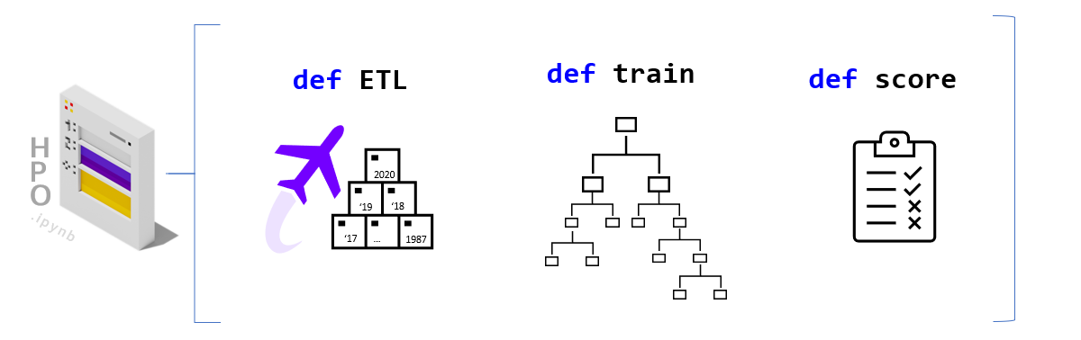
### Dataset
The default settings for this demo are built to utilize the Airline dataset (Carrier On-Time Performance 1987-2020, available from the [Bureau of Transportation Statistics](https://transtats.bts.gov/Tables.asp?DB_ID=120&DB_Name=Airline%20On-Time%20Performance%20Data&DB_Short_Name=On-Time#)). Below are some additional details about this dataset, we plan to offer a companion notebook that does a deep dive on the data science behind this dataset. Note that if you are using an alternate dataset (e.g., NYC Taxi or BYOData) these details are not relevant.
The public dataset contains logs/features about flights in the United States (17 airlines) including:
* Locations and distance ( `Origin`, `Dest`, `Distance` )
* Airline / carrier ( `Reporting_Airline` )
* Scheduled departure and arrival times ( `CRSDepTime` and `CRSArrTime` )
* Actual departure and arrival times ( `DpTime` and `ArrTime` )
* Difference between scheduled & actual times ( `ArrDelay` and `DepDelay` )
* Binary encoded version of late, aka our target variable ( `ArrDelay15` )
Using these features we will build a classifier model to predict whether a flight is going to be more than 15 minutes late on arrival as it prepares to depart.
### Python ML Workflow
To build a RAPIDS enabled SageMaker HPO we first need to build a [SageMaker Estimator](https://sagemaker.readthedocs.io/en/stable/api/training/estimators.html). An Estimator is a container image that captures all the software needed to run an HPO experiment. The container is augmented with entrypoint code that will be triggered at runtime by each worker. The entrypoint code enables us to write custom models and hook them up to data.
In order to work with SageMaker HPO, the entrypoint logic should parse hyperparameters (supplied by AWS SageMaker), load and split data, build and train a model, score/evaluate the trained model, and emit an output representing the final score for the given hyperparameter setting. We’ve already built multiple variations of this code.
If you would like to make changes by adding your custom model logic feel free to modify the **train.py** and/or the specific workflow files in the `workflows` directory. You are also welcome to uncomment the cells below to load the read/review the code.
First, let’s switch our working directory to the location of the Estimator entrypoint and library code.
```ipython3
# %load train.py
```
```ipython3
# %load workflows/MLWorkflowSingleGPU.py
```
## Build Estimator
As we’ve already mentioned, the SageMaker Estimator represents the containerized software stack that AWS SageMaker will replicate to each worker node.
The first step to building our Estimator, is to augment a RAPIDS container with our ML Workflow code from above, and push this image to Amazon Elastic Cloud Registry so it is available to SageMaker.
### Containerize and Push to ECR
Now let’s turn to building our container so that it can integrate with the AWS SageMaker HPO API.
Our container can either be built on top of the latest RAPIDS [ nightly ] image as a starting layer or the RAPIDS stable image.
```ipython3
rapids_base_container = "rapidsai/base:25.12a-cuda12-py3.13"
```
Let’s also decide on the full name of our container.
```ipython3
image_base = "sagemaker-rapids-mnmg-100"
image_tag = rapids_base_container.split(":")[1]
```
```ipython3
ecr_fullname = (
f"{account[0]}.dkr.ecr.{region[0]}.amazonaws.com/{image_base}:{image_tag}"
)
```
#### Write Dockerfile
We write out the Dockerfile to disk, and in a few cells execute the docker build command.
Let’s now write our selected RAPDIS image layer as the first FROM statement in the the Dockerfile.
```ipython3
with open("Dockerfile", "w") as dockerfile:
dockerfile.writelines(
f"FROM {rapids_base_container} \n\n"
f'ENV AWS_DATASET_DIRECTORY="{dataset_directory}"\n'
f'ENV AWS_ALGORITHM_CHOICE="{algorithm_choice}"\n'
f'ENV AWS_ML_WORKFLOW_CHOICE="{ml_workflow_choice}"\n'
f'ENV AWS_CV_FOLDS="{cv_folds}"\n'
)
```
Next let’s append the remaining pieces of the Dockerfile, namely adding dependencies and our Python code.
```ipython3
%%writefile -a Dockerfile
# ensure printed output/log-messages retain correct order
ENV PYTHONUNBUFFERED=True
# install a few more dependencies
RUN conda install --yes -n base \
-c rapidsai-nightly -c conda-forge -c nvidia \
cupy \
dask-ml \
flask \
protobuf \
rapids-dask-dependency=${{ rapids_version }} \
'sagemaker-python-sdk>=2.239.0'
# path where SageMaker looks for code when container runs in the cloud
ENV CLOUD_PATH="/opt/ml/code"
# copy our latest [local] code into the container
COPY . $CLOUD_PATH
WORKDIR $CLOUD_PATH
ENTRYPOINT ["./entrypoint.sh"]
```
```myst-ansi
Appending to Dockerfile
```
Lastly, let’s ensure that our Dockerfile correctly captured our base image selection.
```ipython3
validate_dockerfile(rapids_base_container)
!cat Dockerfile
```
```myst-ansi
ARG RAPIDS_IMAGE
FROM $RAPIDS_IMAGE as rapids
ENV AWS_DATASET_DIRECTORY="10_year"
ENV AWS_ALGORITHM_CHOICE="XGBoost"
ENV AWS_ML_WORKFLOW_CHOICE="multiGPU"
ENV AWS_CV_FOLDS="10"
# ensure printed output/log-messages retain correct order
ENV PYTHONUNBUFFERED=True
# install a few more dependencies
RUN conda install --yes -n base \
cupy \
flask \
protobuf \
'sagemaker-python-sdk>=2.239.0'
# path where SageMaker looks for code when container runs in the cloud
ENV CLOUD_PATH="/opt/ml/code"
# copy our latest [local] code into the container
COPY . $CLOUD_PATH
WORKDIR $CLOUD_PATH
ENTRYPOINT ["./entrypoint.sh"]
```
#### Build and Tag
The build step will be dominated by the download of the RAPIDS image (base layer). If it’s already been downloaded the build will take less than 1 minute.
```ipython3
!docker pull $rapids_base_container
```
```ipython3
!docker images
```
```ipython3
%%time
!docker build -t $ecr_fullname .
```
```ipython3
!docker images
```
#### Publish to Elastic Cloud Registry (ECR)
Now that we’ve built and tagged our container its time to push it to Amazon’s container registry (ECR). Once in ECR, AWS SageMaker will be able to leverage our image to build Estimators and run experiments.
Docker Login to ECR
```ipython3
docker_login_str = !(aws ecr get-login --region {region[0]} --no-include-email)
```
```ipython3
!{docker_login_str[0]}
```
Create ECR repository [ if it doesn’t already exist]
```ipython3
repository_query = !(aws ecr describe-repositories --repository-names $image_base)
if repository_query[0] == "":
!(aws ecr create-repository --repository-name $image_base)
```
Let’s now actually push the container to ECR
> Note the first push to ECR may take some time (hopefully less than 10 minutes).
```ipython3
!docker push $ecr_fullname
```
### Create Estimator
Having built our container [ +custom logic] and pushed it to ECR, we can finally compile all of efforts into an Estimator instance.
```ipython3
!docker images
```
```ipython3
# 'volume_size' - EBS volume size in GB, default = 30
estimator_params = {
"image_uri": ecr_fullname,
"role": execution_role,
"instance_type": instance_type,
"instance_count": 2,
"input_mode": "File",
"output_path": s3_model_output,
"use_spot_instances": use_spot_instances_flag,
"max_run": max_duration_of_experiment_seconds, # 24 hours
"sagemaker_session": session,
}
if use_spot_instances_flag:
estimator_params.update({"max_wait": max_duration_of_experiment_seconds + 1})
```
```ipython3
estimator = sagemaker.estimator.Estimator(**estimator_params)
```
### Test Estimator
Now we are ready to test by asking SageMaker to run the BYOContainer logic inside our Estimator. This is a useful step if you’ve made changes to your custom logic and are interested in making sure everything works before launching a large HPO search.
> Note: This verification step will use the default hyperparameter values declared in our custom train code, as SageMaker HPO will not be orchestrating a search for this single run.
```ipython3
summarize_choices(
s3_data_input,
s3_model_output,
ml_workflow_choice,
algorithm_choice,
cv_folds,
instance_type,
use_spot_instances_flag,
search_strategy,
max_jobs,
max_parallel_jobs,
max_duration_of_experiment_seconds,
)
```
```myst-ansi
s3 data input = s3://sagemaker-rapids-hpo-us-west-2/10_year
s3 model output = s3://sagemaker-us-west-2-561241433344/trained-models
compute = multiGPU
algorithm = XGBoost, 10 cv-fold
instance = ml.p3.8xlarge
spot instances = True
hpo strategy = Random
max_experiments = 100
max_parallel = 10
max runtime = 86400 sec
```
```ipython3
job_name = new_job_name_from_config(
dataset_directory,
region,
ml_workflow_choice,
algorithm_choice,
cv_folds,
instance_type,
)
```
```myst-ansi
generated job name : air-mGPU-XGB-10cv-31d03d8b015bfc
```
```ipython3
estimator.fit(inputs=s3_data_input, job_name=job_name.lower())
```
## Run HPO
With a working SageMaker Estimator in hand, the hardest part is behind us. In the key choices section we already defined our search strategy and hyperparameter ranges, so all that remains is to choose a metric to evaluate performance on. For more documentation check out the AWS SageMaker [Hyperparameter Tuner documentation](https://sagemaker.readthedocs.io/en/stable/tuner.html).
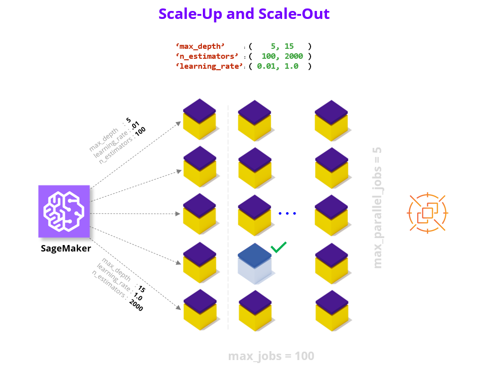
### Define Metric
We only focus on a single metric, which we call ‘final-score’, that captures the accuracy of our model on the test data unseen during training. You are of course welcome to add additional metrics, see [AWS SageMaker documentation on Metrics](https://docs.aws.amazon.com/sagemaker/latest/dg/automatic-model-tuning-define-metrics.html). When defining a metric we provide a regular expression (i.e., string parsing rule) to extract the key metric from the output of each Estimator/worker.
```ipython3
metric_definitions = [{"Name": "final-score", "Regex": "final-score: (.*);"}]
```
```ipython3
objective_metric_name = "final-score"
```
### Define Tuner
Finally we put all of the elements we’ve been building up together into a HyperparameterTuner declaration.
```ipython3
hpo = sagemaker.tuner.HyperparameterTuner(
estimator=estimator,
metric_definitions=metric_definitions,
objective_metric_name=objective_metric_name,
objective_type="Maximize",
hyperparameter_ranges=hyperparameter_ranges,
strategy=search_strategy,
max_jobs=max_jobs,
max_parallel_jobs=max_parallel_jobs,
)
```
### Run HPO
```ipython3
summarize_choices(
s3_data_input,
s3_model_output,
ml_workflow_choice,
algorithm_choice,
cv_folds,
instance_type,
use_spot_instances_flag,
search_strategy,
max_jobs,
max_parallel_jobs,
max_duration_of_experiment_seconds,
)
```
```myst-ansi
s3 data input = s3://sagemaker-rapids-hpo-us-west-2/10_year
s3 model output = s3://sagemaker-us-west-2-561241433344/trained-models
compute = multiGPU
algorithm = XGBoost, 10 cv-fold
instance = ml.p3.8xlarge
spot instances = True
hpo strategy = Random
max_experiments = 100
max_parallel = 10
max runtime = 86400 sec
```
Let’s be sure we take a moment to confirm before launching all of our HPO experiments. Depending on your configuration options running this cell can kick off a massive amount of computation!
> Once this process begins, we recommend that you use the SageMaker UI to keep track of the health of the HPO process and the individual workers.
```ipython3
# tuning_job_name = new_job_name_from_config(dataset_directory, region, ml_workflow_choice,
# algorithm_choice, cv_folds,
# # instance_type)
# hpo.fit( inputs=s3_data_input,
# job_name=tuning_job_name,
# wait=True,
# logs='All')
# hpo.wait() # block until the .fit call above is completed
```
### Results and Summary
Once your job is complete there are multiple ways to analyze the results.
Below we display the performance of the best job, as well printing each HPO trial/job as a row of a dataframe.
```ipython3
tuning_job_name = "air-mGPU-XGB-10cv-527fd372fa4d8d"
```
```ipython3
hpo_results = summarize_hpo_results(tuning_job_name)
```
```myst-ansi
INFO:botocore.credentials:Found credentials from IAM Role: BaseNotebookInstanceEc2InstanceRole
```
```myst-ansi
best score: 0.9203665256500244
best params: {'max_depth': '7', 'max_features': '0.29751893065195945', 'num_boost_round': '346'}
best job-name: air-mGPU-XGB-10cv-527fd372fa4d8d-042-ed1ff13b
```
```ipython3
sagemaker.HyperparameterTuningJobAnalytics(tuning_job_name).dataframe()
```
```myst-ansi
INFO:botocore.credentials:Found credentials from IAM Role: BaseNotebookInstanceEc2InstanceRole
```
For a more in depth look at the HPO process we invite you to check out the HPO_Analyze_TuningJob_Results.ipynb notebook which shows how we can explore interesting things like the impact of each individual hyperparameter on the performance metric.
### Getting the Best Model
Next let’s download the best trained model from our HPO runs.
```ipython3
local_filename, s3_path_to_best_model = download_best_model(
model_output_bucket,
s3_model_output,
hpo_results,
best_hpo_model_local_save_directory,
)
```
```myst-ansi
INFO:botocore.credentials:Found credentials from IAM Role: BaseNotebookInstanceEc2InstanceRole
```
```myst-ansi
Successfully downloaded best model
> filename: /home/ec2-user/SageMaker/cloud-ml-examples/aws/best_model.tar.gz
> local directory : /home/ec2-user/SageMaker/cloud-ml-examples/aws
full S3 path : s3://sagemaker-us-west-2-561241433344/trained-models/air-mGPU-XGB-10cv-527fd372fa4d8d-042-ed1ff13b/output/model.tar.gz
```
### Model Serving
With your best model in hand, you can now move on to [serving this model on SageMaker](https://docs.aws.amazon.com/sagemaker/latest/dg/how-it-works-deployment.html).
In the example below we show you how to build a [RealTimePredictor](https://sagemaker.readthedocs.io/en/stable/api/inference/predictors.html) using the best model found during the HPO search. We will add a lightweight Flask server to our RAPIDS Estimator (a.k.a., container) which will handle the incoming requests and pass them along to the trained model for inference. If you are curious about how this works under the hood check out the [Use Your Own Inference Server](https://docs.aws.amazon.com/sagemaker/latest/dg/your-algorithms-inference-code.html) documentation and reference the code in `serve.py`.
If you are interested in additional serving options (e.g., large batch with batch-transform), we plan to add a companion notebook that will provide additional details.
#### GPU serving
```ipython3
endpoint_model = sagemaker.model.Model(
image_uri=ecr_fullname, role=execution_role, model_data=s3_path_to_best_model
)
```
Kick off an instance for prediction [ recommend ‘ml.g4dn.2xlarge’ ]
```ipython3
DEMO_SERVING_FLAG = True
if DEMO_SERVING_FLAG:
endpoint_model.deploy(
initial_instance_count=1, instance_type="ml.g4dn.2xlarge"
) #'ml.p3.2xlarge'
```
```myst-ansi
INFO:sagemaker:Creating model with name: rapids-sagemaker-mnmg-100-2023-01-23-22-24-22-008
INFO:sagemaker:Creating endpoint-config with name rapids-sagemaker-mnmg-100-2023-01-23-22-24-22-498
INFO:sagemaker:Creating endpoint with name rapids-sagemaker-mnmg-100-2023-01-23-22-24-22-498
```
```myst-ansi
---------!
```
Perform the prediction and return the result(s).
Below we’ve compiled examples to sanity test the trained model performance on the Airline dataset.
> The first example is from a 2019 flight that departed nine minutes early,
> The second example is from a 2018 flight that was more than two hours late to depart.
When we run these samples we expect to see **b’[0.0, 1.0]** as the printed result.
We encourage you to modify the queries below especially if you plug in your own dataset.
```ipython3
if DEMO_SERVING_FLAG:
predictor = sagemaker.predictor.Predictor(
endpoint_name=str(endpoint_model.endpoint_name), sagemaker_session=session
)
if dataset_directory in ["1_year", "3_year", "10_year"]:
on_time_example = [
2019.0,
4.0,
12.0,
2.0,
3647.0,
20452.0,
30977.0,
33244.0,
1943.0,
-9.0,
0.0,
75.0,
491.0,
] # 9 minutes early departure
late_example = [
2018.0,
3.0,
9.0,
5.0,
2279.0,
20409.0,
30721.0,
31703.0,
733.0,
123.0,
1.0,
61.0,
200.0,
]
example_payload = str(list([on_time_example, late_example]))
else:
example_payload = "" # fill in a sample payload
result = predictor.predict(example_payload)
print(result)
```
```myst-ansi
b'[0.0, 1.0]'
```
Once we are finished with the serving example, we should be sure to clean up and delete the endpoint.
```ipython3
# if DEMO_SERVING_FLAG:
# predictor.delete_endpoint()
```
## Summary
We’ve now successfully built a RAPIDS ML workflow, containerized it (as a SageMaker Estimator), and launched a set of HPO experiments to find the best hyperparamters for our model.
If you are curious to go further, we invite you to plug in your own dataset and tweak the configuration settings to find your champion model!
**HPO Experiment Details**
As mentioned in the introduction we find a **12X** speedup in wall clock time and a **4.5x** reduction in cost when comparing between GPU and CPU instances on 100 HPO trials using 10 parallel workers on 10 years of the Airline Dataset (~63M flights). In these experiments we used the XGBoost algorithm with the multi-GPU vs multi-CPU Dask cluster and 10 cross validation folds. Below we offer a table with additional details.
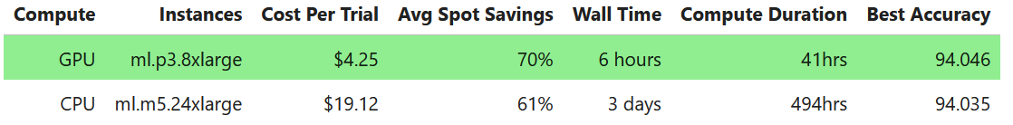
In the case of the CPU runs, 12 jobs were stopped since they exceeded the 24 hour limit we set. CPU Job Summary Image
In the case of the GPU runs, no jobs were stopped. GPU Job Summary Image
Note that in both cases 1 job failed because a spot instance was terminated. But 1 failed job out of 100 is a minimal tradeoff for the significant cost savings.
## Appendix
### Bring Your Own Dataset Checklist
If you plan to use your own dataset (BYOD) here is a checklist to help you integrate into the workflow:
> - [ ] Dataset should be in either CSV or Parquet format.
> - [ ] Dataset is already pre-processed (and all feature-engineering is done).
> - [ ] Dataset is uploaded to S3 and `data_bucket` and `dataset_directory` have been set to the location of your data.
> - [ ] Dataset feature and target columns have been enumerated in `/HPODataset.py`
### Rapids References
> [More Cloud Deployment Workflow Examples](https://docs.rapids.ai/deployment/stable/examples/)
> [RAPIDS HPO](https://rapids.ai/hpo)
> [cuML Documentation](https://docs.rapids.ai/api/cuml/nightly/)
### SageMaker References
> [SageMaker Training Toolkit](https://github.com/aws/sagemaker-training-toolkit)
> [Estimator Parameters](https://sagemaker.readthedocs.io/en/stable/api/training/estimators.html)
> Spot Instances [docs](https://docs.aws.amazon.com/sagemaker/latest/dg/model-managed-spot-training.html), and [blog](https://aws.amazon.com/blogs/aws/managed-spot-training-save-up-to-90-on-your-amazon-sagemaker-training-jobs/)
# index.html.md
# Getting Started with cudf.pandas and Snowflake
*February, 2025*
## RAPIDS in Snowflake
[RAPIDS](https://rapids.ai/) is a suite of libraries to execute end-to-end data science pipelines entirely on GPUs. If you have data in a [Snowflake](https://www.snowflake.com/) table that you want to explore with the RAPIDS, you can deploy RAPIDS in Snowflake using Snowpark Container Services.
## NYC Parking Tickets `cudf.pandas` Example
If you have data in a Snowflake table, you can accelerate your ETL workflow with `cuDF.pandas`. With `cudf.pandas` you can accelerate the `pandas` ecosystem, with zero code changes. Just load `cudf.pandas` and you will have the benefits of GPU acceleration, with automatic CPU fallback if needed.
For this example, we have a Snowflake table with the [Parking Violations Issued - Fiscal Year 2022](https://data.cityofnewyork.us/City-Government/Parking-Violations-Issued-Fiscal-Year-2022/7mxj-7a6y/about_data) dataset from NYC Open Data.
### Get data into a Snowflake table
To follow along, you will need to have the NYC Parking Violations data into your snowflake account, and make sure that this data is accessible from the RAPIDS notebook Snowpark Service Container that you deployed following the [Run RAPIDS on Snowflake](../../platforms/snowflake.md) guide.
In a Snowflake SQL sheet and with `ACCOUNTADMIN` role
```sql
-- Create a database where the table would live --
CREATE DATABASE CUDF_SNOWFLAKE_EXAMPLE;
USE DATABASE DATABASE CUDF_SNOWFLAKE_EXAMPLE;
CREATE OR REPLACE FILE FORMAT my_parquet_format
TYPE = 'PARQUET';
CREATE OR REPLACE STAGE my_s3_stage
URL = 's3://rapidsai-data/datasets/nyc_parking/'
FILE_FORMAT = my_parquet_format;
-- Infer schema from parquet file to use when creating table later --
SELECT COLUMN_NAME, TYPE
FROM TABLE(
INFER_SCHEMA(
LOCATION => '@my_s3_stage',
FILE_FORMAT => 'my_parquet_format',
FILES => ('nyc_parking_violations_2022.parquet')
)
);
-- Create table using the inferred schema in the previous step --
CREATE OR REPLACE TABLE NYC_PARKING_VIOLATIONS
USING TEMPLATE (
SELECT ARRAY_AGG(OBJECT_CONSTRUCT(*))
FROM TABLE(
INFER_SCHEMA(
LOCATION => '@my_s3_stage',
FILE_FORMAT => 'my_parquet_format',
FILES => ('nyc_parking_violations_2022.parquet')
)
));
-- Get data from the stage into the table --
COPY INTO NYC_PARKING_VIOLATIONS
FROM @my_s3_stage
FILES = ('nyc_parking_violations_2022.parquet')
FILE_FORMAT = (TYPE = 'PARQUET')
MATCH_BY_COLUMN_NAME = CASE_INSENSITIVE;
```
### Ensure access from container
During the process of deploying RAPIDS in Snowflake, you created a `CONTAINER_USER_ROLE` and we need to make sure this role has access to the database, schema and table where the data is, to be able to query from it.
```sql
-- Ensure the role has USAGE permissions on the database and schema
GRANT USAGE ON DATABASE CUDF_SNOWFLAKE_EXAMPLE TO ROLE CONTAINER_USER_ROLE;
GRANT USAGE ON SCHEMA CUDF_SNOWFLAKE_EXAMPLE.PUBLIC TO ROLE CONTAINER_USER_ROLE;
-- Ensure the role has SELECT permission on the table
GRANT SELECT ON TABLE CUDF_SNOWFLAKE_EXAMPLE.PUBLIC.NYC_PARKING_VIOLATIONS TO ROLE CONTAINER_USER_ROLE;
```
### Read data and play around.
Now that you have the data in a Snowflake table, and the RAPIDS Snowpark container up and running, create a new notebook in the `workspace` directory (anything that is added to this directory will persist), and follow the instructions below.

### Load cudf.pandas
In the first cell of your notebook, load the `cudf.pandas` extension
```ipython3
%load_ext cudf.pandas
```
### Connect to Snowflake and create a Snowpark session
```ipython3
import os
from pathlib import Path
from snowflake.snowpark import Session
connection_parameters = {
"account": os.getenv("SNOWFLAKE_ACCOUNT"),
"host": os.getenv("SNOWFLAKE_HOST"),
"token": Path("/snowflake/session/token").read_text(),
"authenticator": "oauth",
"database": "CUDF_SNOWFLAKE_EXAMPLE", # the created database
"schema": "PUBLIC",
"warehouse": "CONTAINER_HOL_WH",
}
session = Session.builder.configs(connection_parameters).create()
# Check the session
print(
f"Current session info: Warehouse: {session.get_current_warehouse()} "
f"Database: {session.get_current_database()} "
f"Schema: {session.get_current_schema()} "
f"Role: {session.get_current_role()}"
)
```
```ipython3
# Get some interesting columns from the table
table = session.table("NYC_PARKING_VIOLATIONS").select(
"Registration State",
"Violation Description",
"Vehicle Body Type",
"Issue Date",
"Summons Number",
)
table
```
Notice that up to this point, we have a snowpark dataframe. To get a pandas dataframe we use `.to_pandas()`
#### WARNING
At the moment, there is a known issue that is preventing us to accelerate the following step with cudf, and we hope to solve this issue soon. In the meantime we need to do a workaround to get the data into a pandas dataframe that `cudf.pandas` can understand.
```ipython3
from cudf.pandas.module_accelerator import disable_module_accelerator
with disable_module_accelerator():
df = table.to_pandas()
import pandas as pd
df = pd.DataFrame(df) # this will take a few seconds
```
In the future the cell above will reduce to simple doing `df = table.to_pandas()`.
But now we are ready to get see `cudf.pandas` in action. For the record, this dataset has `len(df) = 15435607` and you should see the following operations take in the order of milliseconds to run.
**Which parking violation is most commonly committed by vehicles from various U.S states?**
Each record in our dataset contains the state of registration of the offending vehicle, and the type of parking offence. Let’s say we want to get the most common type of offence for vehicles registered in different states. We can do:
```ipython3
%%time
(
df[["Registration State", "Violation Description"]] # get only these two columns
.value_counts() # get the count of offences per state and per type of offence
.groupby("Registration State") # group by state
.head(
1
) # get the first row in each group (the type of offence with the largest count)
.sort_index() # sort by state name
.reset_index()
)
```
**Which vehicle body types are most frequently involved in parking violations?**
We can also investigate which vehicle body types most commonly appear in parking violations
```ipython3
%%time
(
df.groupby(["Vehicle Body Type"])
.agg({"Summons Number": "count"})
.rename(columns={"Summons Number": "Count"})
.sort_values(["Count"], ascending=False)
)
```
**How do parking violations vary across days of the week?**
```ipython3
%%time
weekday_names = {
0: "Monday",
1: "Tuesday",
2: "Wednesday",
3: "Thursday",
4: "Friday",
5: "Saturday",
6: "Sunday",
}
df["Issue Date"] = df["Issue Date"].astype("datetime64[ms]")
df["issue_weekday"] = df["Issue Date"].dt.weekday.map(weekday_names)
df.groupby(["issue_weekday"])["Summons Number"].count().sort_values()
```
## Conclusion
With `cudf.pandas` you can GPU accelerated workflows that involve data that is in a Snowflake table, by just reading it into a pandas d
When things start to get a little slow, just load the cudf.pandas and run your existing code on a GPU!
To learn more, we encourage you to visit [rapids.ai/cudf-pandas](https://rapids.ai/cudf-pandas/).